Infinite boundary conditions as Adam Iaizzi 1, * a current source - - PowerPoint PPT Presentation

infinite boundary conditions as
SMART_READER_LITE
LIVE PREVIEW

Infinite boundary conditions as Adam Iaizzi 1, * a current source - - PowerPoint PPT Presentation

APS March Meeting 2019, K19.00003 Infinite boundary conditions as Adam Iaizzi 1, * a current source for impurity Chung-Yu Lo 2 Pochung Chen 2 conductance in a quantum wire Ying-Jer Kao 1 *iaizzi@bu.edu (presenter) 1 National Taiwan University,


slide-1
SLIDE 1

APS March Meeting 2019, K19.00003

Infinite boundary conditions as a current source for impurity conductance in a quantum wire

Adam Iaizzi1,* Chung-Yu Lo2 Pochung Chen2 Ying-Jer Kao1

*iaizzi@bu.edu (presenter)

1National Taiwan University, Taipei, Taiwan 2National Tsing Hua University, Hsinchu, Taiwan

slide-2
SLIDE 2

Adam Iaizzi - iaizzi@bu.edu

Impurity in a LL Wire

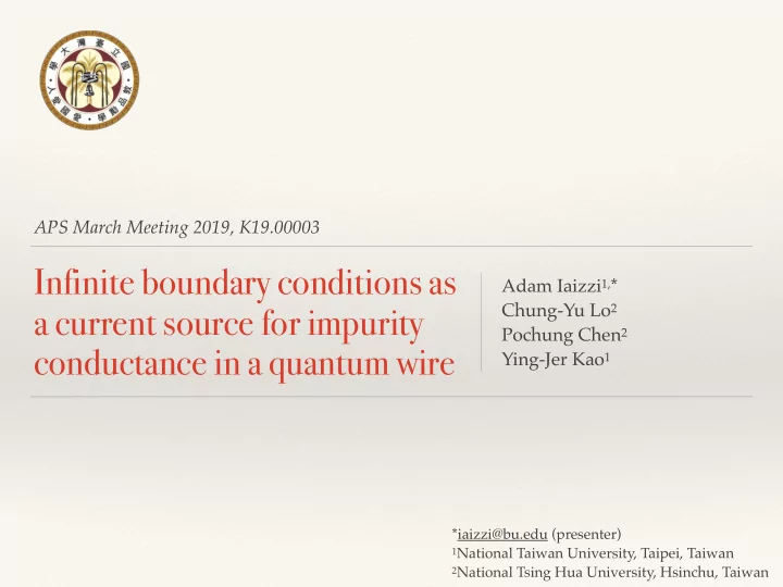
❖ Luttinger liquid wire ❖ Single impurity ❖ Theory: Kane-Fisher ❖ T=0 conductance ❖ g>1 attractive — always

conducts

❖ g=1 noninteracting ❖ g<1 repulsive — always breaks

2

Kane & Fisher PRL 68 1220 (1992)

G ∝ t2V2/g−1

VOLUME 68, NUMBER 8

P H YSICAL REVIEW LETTERS 24 FEBRUARY 1992

e~

4t~

G=-

h

( I+t2)

G=O

e2

G= —

g

h

l It l I I I
  • FIG. 1. Schematic

How diagram

for 1D interacting electrons

with

  • ne

link

weakened by fraction

t.

Here 6 is the conduc- tance across the weak link.

Perfect reflection

is found

for repul-

sive interactions,

g & l, and perfect

transmission for attractive interactions,

g) 1.

Noninteracting electrons, g = I, are mar-

ginal

~

zeroth-order

problem

(t =0) consists of two semi-infinite

lines, which can be described

by the Lagrangian

(3) with

the x integration

restricted to positive

  • r negative

x, re-

spectively.

It is again

convenient

to perform

a partial

trace

(in the p representation), integrating

  • ut p(x) for

all x away from the weakened

link.

We will then obtain

an elfective action

in terms of the phases p+ (r ) on each

side of the link.

If we further

define

P =(P~ — p

)/2 and

4=(p++p

)/2, we may integrate

  • ut 4(r) and obtain

the

following

effective action

in

terms

  • f the

phase difference across the junction:

s„,=g„

I~ I Iy(~) I -'.

(8)

Note that

this expression

is precisely

the

dual

  • f (6).

Again,

we may express

the perturbation t in terms of y,

and the most relevant

  • perator

is

SS—

t

cos[2Jap],

4 z

(9)

I—

t ' (I — e -t")P(V),

  • (IO)

where

the

Fourier transform

  • f P(V), denoted

P(t),

which corresponds

to hopping

an electron across the weak link. In this case the leading-order

RG flows for small

t

are 8t/t)l=(1 —

g

')t, which

is shown

in Fig. 1. Thus,

  • nce again g =1 is marginal,

but now the perturbation

is

irrelevant for g & 1. For repulsively interacting electrons

with g & 1, an initially

weak hopping

scales to zero at low energies.

As shown below, this corresponds

to an insulat-

ing link with strictly zero linear conductance.

This can be seen by deriving

an expression

for the non-

linear current-voltage

characteristics

as a perturbation expansion

in

powers

  • f t.

Upon applying a voltage

V

across the weak link by adding

a vector potential into the argument

  • f the cosine

in (9), we can obtain

an expres- sion for the current

response to second order in t: satisfies

t fF

InP(t) =

dry(2/tag) [coth(Pco/2)( —

1+cosset)

i sintot], where EF is the Fermi energy.

This result

is similar

(but

not identical)

to that obtained

by Devoret

et al. [5] who studied the elfects of a series resistor (modeled

a la Cal-

deira and Leggett [14]) on a tunnel junction.

The boson-

ic excitations

  • f the

Luttinger-liquid leads described

by

(3) are an explicit

physical

realization

  • f the Caldeira-

Leggett oscillators.

In the expression derived by Devoret

et al. , though,

when

the series lead resistance

is set to

zero, an Ohmic I-V curve follows.

In contrast,

as we see below, (10) and (11) only give an Ohmic I Vcurv-e when the electrons

in the ID leads are not interacting

(g= I),

so that the series lead resistance

is h/e

Evaluating

(10) and (11) at T=0 gives

a power-law

I - V curve:

I—

t - V- ~

.

For noninteracting

fermions

(g = I )

this gives the

expected Ohmic conductance,

whereas the expansion

breaks

down

as

V—0 for g & l.

For g & 1, though,

a truly insulating link with

strictly zero linear conductance

is found.

At T~O the linear con- ductance

vanishes as a power

law for g & 1:

(12)

An approximate

interpolation formula

when

both T and

V are nonzero

is I—

t [Im(T+i V)

~

]. Notice that G

in (12) is not proportional

to the square of the tunneling

DOS: p(e=T) — T~+'t~ .

This

is because

the rele- vant DOS for the conductance

is that for tunneling

into the end of a semi-infinite Luttinger

liquid, which varies as

p„.„d(e)-c' ~ '.

Note that for all gal, p,.„d(e) varies

with a diferent

power than the bulk DOS p(c).

For the lattice electron

model

with one weak link, it is

  • f course

possible

to calculate

the two-terminal conduc-

tance for the noninteracting case

(g= I ) for all t One.

finds G =(e-/h)4t /(I+t ). Thus,

in the RG sense, the

line g= I corresponds

to a "fixed line" (see Fig. I).

In view

  • f this

soluble

case,

it seems extremely plausible

[15] that for g&1 one can join together

the RG IIows be- tween the two perturbative regimes

(I —

t and

small t).

This

would imply

that 6=0 for

all t&l when

g & 1,

whereas

G =ge /h for all nonzero

t when g & 1.

Real experiments

will be complicated by the fact that

any one-channel wire must eventually

  • pen

up into wide

leads,

where presumably

Fermi-liquid theory

is applic-

able. This defines

a length

scale L or a time scale L/it,

which

will cut off' the infrared

divergences

associated

with

the Luttinger liquid.

To study

this we consider

an ideal- ized model of an infinite

  • ne-channel

wire with

electron interactions present

  • nly

in the "sample"

with

lxl & L,

but absent

in the (Fermi-liquid)

"leads, " lxl & L.

In the

absence of the weak link, which

we will take to be placed

in the middle of the sample

at x =0, the appropriate

La-

grangian

is given

by (3), but with g depending

  • n

x, be-

l222

slide-3
SLIDE 3

Adam Iaizzi - iaizzi@bu.edu

Impurity in a quantum wire

❖ Noninteracting —> Exact solvable ❖ Small bias —> static DMRG ❖ NonEQ: Experiment quantum simulator for LL wire

+ impurity

❖ Can do finite current ❖ Tunable interactions ❖ Little corresponding theory/numerics ❖ Can we improve with Infinite Boundary Conditions? ❖ Measure finite-bias conductance ❖ Improve stability ❖ Important for nano electronic devices

3

Anthore et al. PRX 8 031075 (2018)

R V C I

1 µm

slide-4
SLIDE 4

Adam Iaizzi - iaizzi@bu.edu

Defining the problem

❖ Start with wires ❖ Impurity ❖ Jordan-Wigner

Transformation

❖ Spinless fermions

—> S=1/2 XXZ

❖ t —> Jx ❖ V —> Jz ❖ μ —> h

4

H = X

i

 −tc†

ici+1 + h.c. + V (ni − 1

2)(ni+1 − 1 2)

  • ❖ For now:

❖ NI leads Jz=0 ❖ NI impurity

Spinless fermions:

H′− ∑

i [Jz(Sz i Sz i + 1) + Jx

2 (S+

i S− i+1 + S− i S+ i+1)]

Spin chain:

slide-5
SLIDE 5

Adam Iaizzi - iaizzi@bu.edu

Finite-Size DMRG

❖ Time-dependent DMRG ❖ Measure finite current ❖ Open boundaries ❖ Conservation laws ❖ Finite-size effects—ringing

5

  • FIG. 4. Color online DMRG results compared to the exact

results for Jt/V obtained using different clusters L and number

  • f states M, with V=0.001. a L=96, b L=64, c L=32, and d

L=16. Note that for L=96 and 64, M=200 shows good qualitative agreement and M300 even shows good quantitative agreement with the exact results. For L=32 and 16, M=200 and 100 already show excellent quantitative agreement with the exact results.

Al-Hassanieh et al. PRB 73 195304 (2006)

20 40 60 80 100 120

Time

  • 0.25
  • 0.2
  • 0.15
  • 0.1
  • 0.05

0.05 0.1 0.15 0.2 0.25

Jl(T)

slide-6
SLIDE 6

Adam Iaizzi - iaizzi@bu.edu

Damped BC

❖ Add “Wilson Chains” w/

exponentially decaying couplings

❖ ‘Soft’ boundary ❖ Steady-state plateaus are

longer

❖ Can we do better? ❖ Infinite boundary conditions

6

Dias da Silva PRB 78 195317 (2008)

10 20 30

τ

0.04 0.08

J(τ)

N=32 Λ=2 N=72 Λ=1 0.1 0.2 0.3 0.4

∆V

0.05 0.1

<J>τ

0.1 0.2 0.3 0.4

∆V

0.5 1

d<J>τ/d(∆V)(2e

2/h)

N=32 Λ=2 N=72 Λ=1

∆V=0.3 ∆V=0.2 ∆V=0.1

(a) (b) (c)

slide-7
SLIDE 7

Adam Iaizzi - iaizzi@bu.edu

Infinite Boundary Conditions

❖ Procedure: ❖ Do iDMRG for bulk wires ❖ Obtain bulk MPO and MPS ❖ Sandwich a finite chain

between fixed bulk tensors

❖ Do finite-size DMRG

7

Phien, Vidal, & McCulloch, PRB 86 245107 (2012)

! # # # $ $ $

|ψi =

% %

&

%

'

% % % % %

! # # # $ $ $ # $ ! #( #( #( $( $( $( #( $(

H =

% %

&

%

'

% % % % )' % )&

# # $ $ # $ #( #( $( $( #( $(

% )& % )' % % )* % )+ %

, , , , ,( ,( ,( ,(

H =

slide-8
SLIDE 8

Adam Iaizzi - iaizzi@bu.edu

Background

8

❖ Source and Drain from IBC ❖ Allow conservation law violations ❖ Open system ❖ Find GS of finite-size system ❖ T=0, turn on field (ΔV —> Δμ —> Δh) ❖ Time evolve with TEBD

Source V=+ΔV/2 Drain V=-ΔV/2

Impurity Quantum wire Quantum wire

slide-9
SLIDE 9

Adam Iaizzi - iaizzi@bu.edu

Charge density

9

10 20 30 40 50 60

x

  • 0.4
  • 0.3
  • 0.2
  • 0.1

0.1 0.2 0.3 0.4

(Charge Density)/ Step function charge density L=60, BD=20, IBC

=0.001 =0.01 =0.1 Impurity

10 20 30 40 50 60

x

  • 4
  • 3
  • 2
  • 1

1 2 3 4 5

Charge Density

10-4

L=60, BD=20, IBC

uniform =0 uniform = 0.001 Step func. = 0.001 Impurity

slide-10
SLIDE 10

10

slide-11
SLIDE 11

Next steps

❖ Mitigate reflections at boundaries ❖ Better understand IBC as reservoir ❖ Add interacting impurity/QD ❖ Make wires interacting ❖ More impurities or more complex impurities

11

slide-12
SLIDE 12

Thanks

  • Prof. Pochung Chen

National Tsing Hua University

  • Prof. Ying-Jer Kao

National Taiwan University

Chung-Yu Lo

National Tsing Hua University

12

slide-13
SLIDE 13

Contact:

Adam Iaizzi email: iaizzi@bu.edu web: www.iaizzi.me Get started with uni10 uni10.org

Thanks for your attention!

Plug:

Postdocs graduate students

Join FECS!

A new APS unit for early career scientists

(talk to me after)