Modern Hadron Spectroscopy : Challenges and Opportunities Adam - - PowerPoint PPT Presentation

INDIANA UNIVERSITY

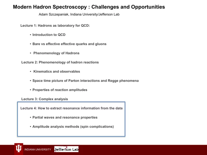
Lecture 1: Hadrons as laboratory for QCD:

• Introduction to QCD
• Bare vs effective effective quarks and gluons
• Phenomenology of Hadrons

Lecture 2: Phenomenology of hadron reactions

• Kinematics and observables
• Space time picture of Parton interactions and Regge phenomena
• Properties of reaction amplitudes

Lecture 3: Complex analysis Lecture 4: How to extract resonance information from the data

• Partial waves and resonance properties
• Amplitude analysis methods (spin complications)

Modern Hadron Spectroscopy : Challenges and Opportunities

Adam Szczepaniak, Indiana University/Jefferson Lab

INDIANA UNIVERSITY

Constructing partial waves (from singularities) 2

K-matrix K-matrix with Chew-Mandelstam “phase space” N/D Coupled channels Flatte formula Isobar model Kinematical singularities (example) Veneziano Amplitude

INDIANA UNIVERSITY

Accessing QCD resonances

3

Veff(R) ∼ Z ψ1ψ2VQ ¯

Qψ3ψ4

T = Veff + X

n

Veff |nihn| E En Veff + · · ·

Effective potential between meson

High spin/mass resonances generated by confining VQQ interact with multi-hadron intermediate states and screen the quark- antiquark potential Both potentials produce ∞ number of poles ! (poles cannot disappear) Confined : ∞ n number of bound states in the

• continuum. No parton production thresholds

Screened : Large decay withers to mupltipartilce finals states (cover rapidity gap in inclusive production)

INDIANA UNIVERSITY

Accessing QCD resonances

4

e.g. for harmonic oscillator confinement E = 2n + l

INDIANA UNIVERSITY

Accessing QCD resonances

5

Coupling to multi-hadron asymptotic states increases with mass/spin of the resonance

INDIANA UNIVERSITY

Scattering through resonances

6

∞ number of poles As energy increases Γ(E) receives contributions from intermediate states with an increasing number of hadrons.

INDIANA UNIVERSITY

7

One resonance, (e.g. ρ) decaying to 2π (µ=0.134) gives a pole at √s=0.767 − 0.056 (on IInd sheet)

Γ(s) Contains effects of multi particles thresholds

f(E) = Πr ⇣ −

g2

r

E−Er

⌘ 1 − iΠrkr ⇣

−g2

r

E−Er

⌘ g2 f(s) = (0.772 − i0.12 p 4 × 0.1342 − s) − s

f(s) = 1 K−1(s) − iΓ(s)

K−1 = Πr(E − Er)

K(s) has (∞ number of) poles

INDIANA UNIVERSITY

8

With ∞ number of resonances this formula doesn’t make sense f(s) → 0 K-1(s) needs to have ∞ number of poles (K(s) needs zeros) Example Linearly spaced radial trajectories (Veneziano) Quadratically spaced radial trajectories

K(s) =

∞

X

r=1

g2

r

m2

r − s →

X

r

1 r2 − s ∼ cos(π√s) sin(π√s)

K(s) ∼ Γ(a−s)

Γ(b−s)

INDIANA UNIVERSITY

Unitarization

9

K(s) has poles and zeros Phase space, besides unitarity branch point has spurious singularities

K(s) = P(s) Q(s)

Zeros Poles

f(s) = K(s) 1 − iK(s)ρ(s)

f(s) = P(s) Q(s) − 1

π

R

str ds0ρ(s0) P (s0) s0s

f(s) = cos(πs) sin(πs) − 1

π

R

str ds0ρ(s0) cos(πs0) s0s

If P(s) has ∞ of zeros it is necessary to “divide” out asymptotic behavior

f(s) =

1 Γ(bs) 1 Γ(as) − 1 π

R

str ds0ρ(s0) 1 Γ(bs0)(s0s)

f(s) =

1 Γ(bs) 1 Γ(as) − sb+s π

R

str ds0ρ(s0) (s0)bs0 Γ(bs0)(s0s)

“Almost correct”, need to remove phases)

INDIANA UNIVERSITY

Other effects

10

Non-quark model resonances (tetraquarks) Yukawa exchange (possibly relevant of when pion exchange)

INDIANA UNIVERSITY

Relativistic case

12

E s s

s = (p1 + p2)2 = ( q p2 + m2

1 +

q p2 + m2

2)2

str = (m1 + m2)2 From u/t channel

INDIANA UNIVERSITY

Other effects of partial wave analyticity

13

Al(s) = Z dzsA(s, t(s, zs), u(s, zs))Pl(cos θ)

Scalar particle scattering 1+2 -> 3 + 4

∝ (m2

e − t(s, zs))−1

t = −(s − 4m2) 2 (1 − zs)

A0(s) ∼ Z 1

−1

dzs 1 m2

e + (s−4m2) 2

(1 − zs)

Partial waves have “right hand” singularity (from s) and “left hand” (from t and u) For example assume equal masses For s>4m2 integral is finite For s<4m2 - me2 the detonator crosses 0 within integration limi, implying A0(s) has a cut for negative s Scalar amplitudes have simple singularity structure, but partial waves a much more

• complicated. They also have kinematical singularities when spin and/or unequal masses

are involved

INDIANA UNIVERSITY

Bound states and Virtual States

14

bound state : pole on the physical energy plane

II(-)

• f0(980),
• a0(980),
• a1(1420),
• Lambda(1405),
• XYZ,
• …

3S 1S

V(r) r

3S 1S

Deuteron the np molecule bound by meson exchange forces

virtual state : pole on “unphysical sheet” closest the physical region thresholds “cut” the physical energy plane

• Thresholds are “windows” to

singularities (particles, visual states, forces” ) located on the nearby unphysical sheet.

• They appear as cusps (if below

threshold) or bumps (is above) Threshold

INDIANA UNIVERSITY

Example : B-> J/psi K pi

15

1 2 3 4 J/Ψ(1) B(2) → K(3) π(4) : s-channel J/Ψ(1) K(3) → B(2) π(4) : t-channel J/Ψ(1) π(4) → K(3) B(2) : u-channel _ _ B(2) → J/Ψ(1) K(3) π(4) : decay _ _ _

INDIANA UNIVERSITY

Veneziano model and application to Dalitz plot analysis

Adam Szczepaniak, Indiana U./JLab

Historical role Properties Application to J/ψ → 3π decays Generalizations (dual models)

INDIANA UNIVERSITY

INDIANA UNIVERSITY

ψ’ J/ψ

BESIII, Phys.Lett. B710 (2012) 594-599

“standard” (isobar)

manifestation of force - particle duality ?

A(s, t) = Γ(−J(s))Γ(−J(t)) Γ(−J(s) − J(t))

dual model

J/ψ

dual model

PRELIMINARY

ψ’

ω → 3π

INDIANA UNIVERSITY

• Duality: resonances in direct channel dual to reggeons in cross

channels and backgrounds are dual to the pomeron

• All resonances are “connected”: resonances belong to Regge

trajectories (reggeons)

• Asymptotics: determined by Regge poles
• Unitarity: imaginary parts determined by decay thresholds

Properties: Veneziano amplitude satisfies all of the above except unitarity, which implemented in the Szczepaniak- Pennington model

INDIANA UNIVERSITY

Veneziano amplitude: “compact” expression for the full

amplitude A(s,t) can be written as sum over resonances in ether channel. Note: in V-model resonance couplings, β, are fixed!

resonance/reggeon in s=m122 β(t) [k - α(s)] _______ ~ B.W. propagator resonance/reggeon in t=m232 β(s) [k - α(t)] _______

A(s, t) = Γ(−α(s))Γ(−α(t)) Γ(−α(s) − α(t)) A(s, t) = X

k

βk(t) k − α(s) = X

k

βk(s) k − α(t) βk(t) ∝ (1 + α(t))(2 + α(t)) · · · (k + α(t)) α(s) = a + bs

INDIANA UNIVERSITY

s1 s2 s3 s4 s5 s6 s l 1 2 3 4 5 leading 1st 2nd 3rd

• r meson with momentum p and

, V (p, ) → ⇡i(p1)⇡j(p2)⇡k(p3)

A(s, t, u) = ✏ijk✏µναβ✏µ(p, )pν

1pα 2 pβ 3

×[An,m(s, t) + An,m(s, u) + An,m(t, u)]

An,m(s, t) ≡ Γ(n − ↵s)Γ(n − ↵t) Γ(n + m − ↵s − ↵t).

and confinement pr ↵(s) = ↵0 + ↵0s. singularities of A

n ≥ m ≥ 1 Regge limit no-double poles

α(s) = 1 2 + s

INDIANA UNIVERSITY

Resonances couplings, β, should depend on final state particles: a linear superposition of

Veneziano amplitudes can be used to suppress or enhance individual resonances or trajectories

s1 s2 s3 s4 s5 s6 s l 1 2 3 4 5 leading 1st 2nd 3rd s Re α(s) Re α(s) = a + b s ρ(770 ρ(1450) ρ(1570 ρ3(1690 ρ ρ3(1990) ρ ρ3 ρ5 M = ✏µναβpµ

1pν 2pα 3 ✏βA(s, t, u)

A = X

n,m

cn,m  Γ(n − α(s))Γ(n − α(t)) Γ(n + m − α(s) − α(t)) + (s, u) + (t, u)

• even-spin ρ’s do not couple

to π π and should decouple in J/ψ→3 π

• coupling of odd-spin ρ’s

depend of can depend vary depending on trajectory

INDIANA UNIVERSITY

An,m(s, t) =

∞

X

k

β(t) k − α(s) =

∞

X

k

β(s) k − α(t)

how to remove (infinite) number of poles? A1,1 = Γ(1 − αs)Γ(1 − αt) Γ(2 − αs − αt) has poles at αs=1,2,3,...

A2,1 = Γ(2 − αs)Γ(2 − αt) Γ(3 − αs − αt)

have poles at αs=3,4,5,...

A2,2 = Γ(2 − αs)Γ(2 − αt) Γ(4 − αs − αt)

have poles at αs=2,3,4,...

A3,1, A3,2, A3,3

A4,1, A4,2, A4,3, A4,4

s t have poles at αs=4,5,6,... n ≥ m ≥ 1 Use a linear combination of A2,1 and A2,2 to remove pole at αs =2 Use a linear combination of A3,1, A3,2 ,A3,3, to remove pole at αs =3, etc.

INDIANA UNIVERSITY

An,m(s, t) → A(s, t) = X

n≥1,n≤m≤1

cn,mAn,m(s, t)

cn,1 = c1,1 Γ(n), cn,2 = − c1,1 Γ(n − 1), cn,m = 0 for m > 2, (10)

A1(s, t) = c1,1 2 − αs − αt (1 − αs)(1 − αt).

remove all poles but the one at α=1 ... but the Regge limit is now lost ! remove all poles between N ≥ α ≥ 2

ain A1(s, t; N) = c1,1 2 − αs − αt (1 − αs)(1 − αt) × Γ(N + 1 − αs)Γ(N + 1 − αt) Γ(N)Γ(N + 2 − αs − αt)

has Regge limit is for s > N

INDIANA UNIVERSITY

The Szczepaniak-Pennington model does this in a systematic way. In addition it allows for imaginary non-linear (and complex) trajectories without introducing “ancestors” In the past this was done by choosing an arbitrary set of n,m and fitting c(n,m) to the data (e.g. Lovelace, Phys. Lett. B28, 265 (1968),Altarelli, Rubinstein,

• Phys. Rev. 183, 1469 (1969))

n: number of Regge trajectories an,i: determine resonance couplings N: determines the onset of Regge behavior α(s), α(t) = Re α + i Im α: with Im α related to resonance widths

INDIANA UNIVERSITY

An(s, t; N) = an,0 2n − αs − αt (n − αs)(n − αt) ⇥ Πn1

i=1 (an,i − αs − αt)

⇤ × Γ(N + 1 − αs)Γ(N + 1 − αt) Γ(N + 1 − n)Γ(N + n + 1 − αs − αt) (15)

All poles below α = N except at α = n s t αs = n αt = n at αs=n residue is a polynomial in t of order n-1 (remember to add 1 from the Levi-Civita tensor)

A(s, t, u) = ✏ijk✏µναβ✏µ(p, )pν

1pα 2 pβ 3

×[An,m(s, t) + An,m(s, u) + An,m(t, u)]

A1 has ρ(770) A3 has ρ(1700), ρ3(1690) A5 has ρ’’(2150), ρ3(2250), ρ5(2350)

INDIANA UNIVERSITY

s1 s2 s3 s4 s5 s6 s l 1 2 3 4 5 leading 1st 2nd 3rd

ρ(1400)

m2 = √s2 = r 2 − 1 2 = 1.23

ρ(1900), ρ3(1990),

m4 = √s4 = r 4 − 1 2 = 1.87

INDIANA UNIVERSITY

4 e, y e ρ e , s

• le

le s, ) 16) 17) ) is e

• = 1

1.5 1.7 1.9 100 150 200 250 1 2 3

M2

200 400 600 800

Events 10

3/2.4MeV

• FIG. 2: Dalitz plot projection of the di-pion mass distribution

from J/ψ decay. The solid is the result of the fit with three amplitudes and the dashed line with the amplitude A1 alone. The insert shows the mass region of the ρ3 and its contribution from the fit with the full set of amplitudes (solid line) as

• compared. Absence of the structure at 1.7GeV from the fit

with the A1 amplitude is indicated by the dashed line.

• = 1
• r

s 18) y s 19) s d )]

• 1

2 3 4

M2

1 2

Events 10

3/ 2.4MeV

• FIG. 3: Dalitz plot projection of the di-pion mass distribution

from ψ0 decay. The solid is the result of the fit with three amplitudes and the dashed line is the fit with A1 alone.

B5 amplitude: Reggeons/ Resonances in all 5 channels

INDIANA UNIVERSITY

Amplitude analysis of the Zc(3900)

31

• Reactions Y(4260) -> J/Ψππ and Y(4260) -> DD*π
• Amplitude is an analytical function of s, the J/Ψπ mass2
• Two coupled channels -> 4 Riemann sheets of A(s) (S-wave partial wave)

t/u channel exchange close to the s-channel physical region (Cusps in the s-channel) s channel exchange close to the s- channel physical region (Resonance bumps in the s-channel)

INDIANA UNIVERSITY

Singularity structure

32

INDIANA UNIVERSITY

The fit I

33

• no t/u channel singularities + s-channel pole

III sheet resonance pole

INDIANA UNIVERSITY

The fit II

34

• u-channel cusp + s-channel pole ((III sheet)

III sheet resonance pole enhanced by the cusp

INDIANA UNIVERSITY

The fit III

35

• t/u channel singularities + no s-channel pole

IV sheet pole from “meson- meson” interactions enhanced by the cusp

INDIANA UNIVERSITY

The fit IV

36

• t/u channel singularities + no s-channel pole

Pure III sheet branch point from u- channel exchanges

INDIANA UNIVERSITY

Where do cusp come from

37

• Possible amplitude singularities are determined by analyticity and unitarity
• No singularities on the physical (Ist sheet)
• At fixed, physical t, growth in s is limited in all directions in

the complex plane

• Poles, sqrt, of log-branch points

A popular Quark Model motivated(*) amplitude behaves like exp(-q2)

• r A(s) ~ exp(-s)

q= | relative 3-momentum | q Such amplitude violates analyticity (*) From overlap of four Gaussian wave functions representing confined quark- anit quark pairs

INDIANA UNIVERSITY

An unphysical cusp effect

38

Ampl ∝ Z

4

ds0 r 1 − 4 s0 N(s0) s0 − s

N(s) ∝ exp(−s)

INDIANA UNIVERSITY

Identification of Resonances

39

Comment on spin formalism

• Analyticity means to explore singularities. There are kinematical and

dynamical singularities

• Kinematical singularities are due to spin and mass differences (e.g. pseudo

thresholds)

• Helicity, Spin-Oribt, Zemach tensors, Chung’s relativistic corrections,

covariant LS by Fillipini et al, Bonn-Gatchina, … : a confusing state of affairs

• Introduce model dependent s,t,u factors
• Do not isolate kinematical singularities
• Do not satisfy crossing
• …..