Juggling Slide Rules By Colin Tombeur December 2011 INTRODUCTION - - PDF document

C Tombeur Page 1 December 2011

Juggling Slide Rules

By Colin Tombeur December 2011

INTRODUCTION

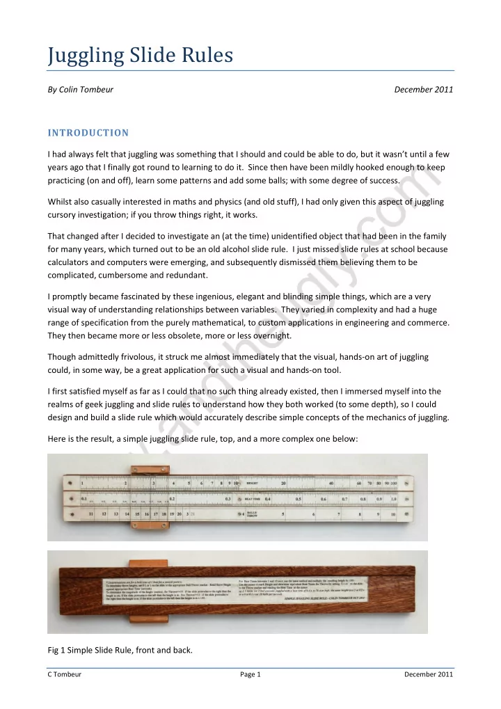
I had always felt that juggling was something that I should and could be able to do, but it wasn’t until a few years ago that I finally got round to learning to do it. Since then have been mildly hooked enough to keep practicing (on and off), learn some patterns and add some balls; with some degree of success. Whilst also casually interested in maths and physics (and old stuff), I had only given this aspect of juggling cursory investigation; if you throw things right, it works. That changed after I decided to investigate an (at the time) unidentified object that had been in the family for many years, which turned out to be an old alcohol slide rule. I just missed slide rules at school because calculators and computers were emerging, and subsequently dismissed them believing them to be complicated, cumbersome and redundant. I promptly became fascinated by these ingenious, elegant and blinding simple things, which are a very visual way of understanding relationships between variables. They varied in complexity and had a huge range of specification from the purely mathematical, to custom applications in engineering and commerce. They then became more or less obsolete, more or less overnight. Though admittedly frivolous, it struck me almost immediately that the visual, hands-on art of juggling could, in some way, be a great application for such a visual and hands-on tool. I first satisfied myself as far as I could that no such thing already existed, then I immersed myself into the realms of geek juggling and slide rules to understand how they both worked (to some depth), so I could design and build a slide rule which would accurately describe simple concepts of the mechanics of juggling. Here is the result, a simple juggling slide rule, top, and a more complex one below: Fig 1 Simple Slide Rule, front and back.

C Tombeur Page 2 December 2011

Fig 2 Complex Slide Rule, front and back. The rest of this document contains the following:  Some Juggling Theory Made Easy  The Simple Juggling Slide Rule; description and instructions.  The Complex Juggling Slide Rule; description and instructions.  Construction  Variables and Formulae Used  Printable scales from the rules. The text is written with both juggling and slide rule communities in mind, and whilst I have tried to make it as accessible as possible, it is inevitable that parts may be either somewhat basic or too complicated, depending on the reader’s interests. Also, as I decided that to best understand the mechanics of juggling I would work out the theory myself and then seek corroboration and further insight, some of my terminology may conflict with what is already ‘out there’. That all said, I hope the reader will find the rest of this text at least a little bit interesting…

C Tombeur Page 3 December 2011

SOME JUGGLING THEORY MADE EASY (!?)

Ultimately, whilst the physics and maths may be a little complicated, for my purposes and for the juggler juggling a number of balls with 2 hands throwing alternately (most common patterns fit this criteria) there are really only 4 interrelated things to worry about: The weight of the throw; ie its siteswap or when it is next thrown (or number of balls in a regular cascade/fountain pattern where all throws are the same). The height of the throw (meters). The throw rate, or beat (seconds). How long the object is held on to between catching and throwing it (hold, wait or dwell time, in beats). Any three of these will determine the fourth, the relationships can be explored and comparisons between different values made. Then with the inclusion of the distance between the throw and catch sites all sorts of things can be calculated, down to the number of Mars bars need to keep a 5 ball cascade running for an hour if you wanted. A little juggling theory is necessary, but in keeping with the practical approach and application to a simple tool, I will attempt to be concise. I have also tried to avoid formulas and complex notation, except for reference in the appendix. Thinking of a simple 3 ball cascade, each ball is thrown the same but in alternating directions, hand to hand. So each ball has the pattern in time, which fit together into a smooth running pattern of throws and catches. Each ball is thrown, it flies and it is caught. The catch to throw can be thought of as one part of the time pattern and the flight (air time) another. For a smooth pattern the throws are regular, and the time from

• ne to the next is called a BEAT. For simplicity I also measure the wait time in beats.

Since each of the three balls is thrown the same, consecutively, then each ball is next thrown 3 throws (or beats) later, so the weight of each throw is said to be a ‘3’. The ratio of flight time to wait time can vary, but in theory it can be seen that the ‘neatest’ pattern is where the flight time is twice as long as the wait time and each hand is empty as long as it is full (fig 3(. In this case the wait time is one beat, so I call this the base (1) of a throw. Although in theory this timing is the neatest, in practice a smooth, comfortable pattern is achieved at wait times nearer 1.5 beats. In fact it can be seen that wait times can be between 0 and 2 beats (fig 4). This is important as the longer the wait time, the shorter the air time and consequently the lower the throw. Fig 3, 3 ball cascade at wait = 1 beat.

beat 1 2 3 4 5 6 R L R L R L R L Ball 3 Ball 2 Ball 1 wait = 1 beat

C Tombeur Page 4 December 2011

Fig 4, 3 ball cascade at wait = 0 beats (throw immediately, hands almost always empty), and wait = 2 beats (throw as next ball is caught, hands almost always full). The weight of the throw minus the wait time (in beats) gives the air time (again in beats), which for a given throw rate (beats per second or seconds per beat) will give the height of the throw. Similarly for certain heights, throw rates can be determined, dependant on the weight. This theory for the 3 ball cascade (where all throws are weight 3) is valid for any weight of throw in a juggle- able pattern of any number of balls (and gaps) where the throws are regular and made by alternate hands. For example a [weight] 5 throw (which would be used solely to keep a regular 5 ball cascade going), at a certain beat and wait time, determines its height, or the height is determined the throw rate and hold. At base 1 (wait = 1 beat) it can easily be seen that for the same beat time, a 5 has twice the air time of a 3, and hence (due to the laws of physics ) is four times as high. Conversely, the pattern must be juggled twice as fast if the height is the same. Incidentally it can easily be seen here that an odd weighted throw is always caught by the opposite hand (from where it will subsequently be thrown back again), and an even numbered throw is caught by the same hand that threw it, although this is more relevant when designing and actually juggling patterns. The simple interrelation of these 4 variables within the laws of projectile motion can easily be applied to a mechanical device with scales, where their relationships can easily be seen and magnitudes determined.

beat 1 2 3 4 5 6 R L R L R R L Ball 3 Ball 2 Ball 1 wait = 0 beat beat 1 2 3 4 5 6 R L L R R L R R L R R L L Ball 3 Ball 2 Ball 1 wait = 2 beat

C Tombeur Page 5 December 2011

THE SIMPLE JUGGLING SLIDE RULE

The simple juggling slide rule was the first application of this theory, designed for base 1 (wait time = 1 beat) throws to calculate heights and show equivalents. It was kept simple to test both the theory and my craftsmanship (or lack thereof). It has just 3 scales as follows :  Height – at the top of the body, which can be read in centimetres or metres as appropriate.  Beat Time – on the slide, from 0.1 to 1 second (can be used from 1 to 10 seconds also).  Balls/Throw – a marker scale at the bottom of the body to index the weight of the throw (or number of balls in a regular pattern). From a slide rule perspective, the Height scale is simply an A scale (logarithmic 1 to 100), and the Beat Time scale is a C scale (logarithmic 1 to 10, labelled as 0.1 to 1.0). This is because the height of a throw is proportional to the square of the time it is in the air. By setting 0.1 (or 1.0 as appropriate) on the slide to the Ball/Throw marker on the bottom scale, the Height

• f the throw on the top scale can then be read against the required Beat Time on the slide. The line on the

cursor can be used to make readings easier if required. Fig 5 For example, by setting 0.1 on the slide to the 3 ball/throw marker (fig 5), heights of 4.9cm, 19.6cm, 44.1cm and 78.4cm can be read against beat times of 0.1second (10 throws per sec), 0.2s, 0.3 and 0.4s respectively. It can also easily be seen from fig 5, that a weight 3 thrown at 0.2s beat time is the same height as a weight 5 at 0.1s, since the 5 marker lines up exactly. Similarly it can be seen that a 7 at 0.1s is the same as a 3 at 0.3s, or an 8 at 0.1s is the same as a 3 at 0.35s. Fig 6 Fig 6 shows that the height of a 5 at 0.4s beat time (2.5 throws per sec) is 3.14m, which is the same height

• f a 17 at 0.1s.

C Tombeur Page 6 December 2011

There are simple rules to determine the magnitude of the height as follows :  For throws less than or equal to 10, if the slide protrudes to the right then the height is cm.  For throws less than or equal to 10, if the slide protrudes to the left then the height is m.  For throws greater than or equal to 11, if the slide protrudes to the right then the height is m.  For throws greater than or equal to 11, if the slide protrudes to the left then the height is m x 100. An abbreviated form of these instructions is on the back of the slide (see fig 1). It is possible to do more complicated comparisons, for example by setting 1.0 on the slide to weight 5 and positioning the cursor at 0.35s, the height is marked. Reposition the slide to 1.0 at weight 8 and the cursor will be at 0.2s on the slide. So a weight 5 at a beat of 0.35s is the same height as a weight 8 at 0.2s (figs 7 & 8). Fig 7 Fig 8 A simple way to read equivalents of height or speed (at wait =1 beat) is to set 0.1s (or 1.0s) on the slide to the lower weight, and reading the number (ignoring the decimal) on the slide corresponding to the higher

• weight. For example, set 0.1 to throw 4 and read 3 at throw 10, this means that for any height the regular

pattern of throw 10 is three times faster than that of throw 4 (fig 9). Fig 9 The square of this is the factor of height difference if the patterns are juggled at the same speed, in this case 9 times higher. A simple way to calculate the square is to align the Beat Time scale exactly with the Height scale and simply read from one to the other, ignoring the decimal (fig 1).

C Tombeur Page 7 December 2011

THE COMPLEX JUGGLING SLIDE RULE

The Complex Juggling Slide rule allows more sophisticated calculations to be made and relationships explored, in the world of juggling mechanics. It has the 3 basic scales of the Simple rule, though differently laid out and labelled, plus other custom juggling scales and some standard slide rule scales for a broad scope of calculations. The rule has nine scales in total, two at the top of the body, four on the slide and three on the bottom of the body, labelled and described as follows:  n1 (green) : custom marker scale for the base of the throw value or weight (n from 2 to 21) where wait time is 1 beat  A scale, also labelled h : standard slide rule A scale (logarithmic 1 to 100) for calculations and where height (h) is read.  C-1 scale, also labelled ns-1 : standard slide rule inverse C scale (logarithmic 10 to 1) for calculations and used for throw rate (f) in balls (or throws, n) per second.  sin-1θ scale (red) : custom inverse sin scale (corresponds to C-1 scale x10-1).  n(wb) scale (green) : custom scale of markers of throw value (n from 2 to 11) with scales of wait times in beats (wb) indicated for each throw. The precise fractional component of the wait time can be read on the C scale.  C scale, also labelled t and bt x10-1 : standard slide rule C scale (logarithmic 1 to 10) for calculations and where beat time (b) is read in tenths of a second, and air time is (t) is read.  D scale, also labelled v : standard slide rule D scale (logarithmic 1 to 10) for calculations and where max velocity (v) and vertical velocity (vy) is read.  A-1 scale (blue), also labelled d-1 x10-2m : standard slide rule inverse A scale (logarithmic 100 to 1) for calculations and where distance between hands (d) is read in cm.  θ scale (blue): custom 2 line scale to determine the angle (θ) from the horizontal that balls are thrown. There are markers on the C and D scales for π (3.1412) and g (9.81ms-1), and on the C scale for vertical velocity (vy). Normal slide rule calculations can be done using the A, A-1, C, C-1, D and sin-1θ scales, and the hairline

• n the cursor (X) can be used to aid alignments or mark values.

A summary of instructions is on the reverse of the slide rule (fig 2). Determinations of throw height are made in a similar way to the Simple rule, however the speed of throws can either be defined as beat time using the C scale , or throws per second using the inverse C scale, eg 5 throws per second on the C-1 is 0.2s on the C scale. Either the left or right end of the slide is aligned with the throw weight on the n1 scale, the cursor can then be used to mark the height on the h scale for base 1 of the weight (wait time =1 beat). Heights for different wait times can be determined by positioning the weight base 1 mark on the n(wb) scale on the slide to the cursor hairline, and reading h against n(wb) for weight time between 0 and 2 beats for the weight.

C Tombeur Page 8 December 2011

For example (figs 10 & 11), position 10 on the C-1 scale against 4 marker on the n1 scale, and position the cursor at 5 on the C-1 scale, the height 44.1cm can then be read on the h scale as the height of a weight 4 throw at wait time of 1 beat where the throw rate is 5 balls per second. Position 4(1) on the n(wb) scale to the cursor hairline and then read h for different wait times between 0 and 2 beats (using fractional markings in the C scale for accuracy); at 2 beats 19.6cm, at 0 beats 78.4cm, at 1.5 beats 30.6cm etc. Fig 10 Fig 11 Rules for determining the magnitude of the height for a beat time between 0.1 and 1 second (1 to 10 throws per second) are the same as the Simple rule, for beat times between 1 and 10 seconds the height determined must be factored up by 100. The inclusion of the n(wb) and D scales make it very easy to compare throw speeds and heights of different weights and wait times. Set the slide so the first throw(wait) on the n(wb) scale is aligned to the 1 on the D scale, then against the comparison throw(wait) on the n(wb) scale either read the multiple of throw rate on the D scale (for the same height) or the height multiple on h for the same throw rate. Fig 12 Fig 12 shows that for the same height, compared to a 3 throw (wait = 1 beat), a 5 (wait = 1 beat) the beats would be twice as fast, a 9 (wait = 1 beat) the beats four times as fast. Similarly for the same beat speed the heights would be 4 and 16 times higher respectively.

C Tombeur Page 9 December 2011

Fig 13 Fig 13 shows that for the same height, compared to a 3 throw (wait = 1.5 beat), a 5 (wait = 1.5 beat) the beats would be 2.33 times as fast, a 9 (wait = 1.5 beat) the beats five times as fast. Similarly for the same beat speed the heights would be 5.45 and 25 times higher respectively. The air time (t) of a throw is simply the beat time (b) multiplied by the weight (n) of the throw minus the wait time in beats (wb). This can be calculated using the standard slide rule scales (C and D) and

• methodology. (Briefly, set 1 (or 10) on the C scale to the beat time on the D scale, find the number of

beats of air time (weight minus wait beats) on the C scale and read the answer on the D scale against it. Determine the magnitude in seconds by inspection. ExampleFig 14.) Fig 14 Sile rule calculation 2 x 4 = 8 ! The throw angle to the horizontal (θ) for a throw width (d) and air time (t), assuming throw and catch sites are level, is calculated by setting 1 (or 10 as appropriate) on the C scale to the throw width on the A-1 scale, then reading the angle on the θ scale against the air time in seconds on the C scale accoring to the following rules:  If 0<= t <=1 second, d is cm and slide protrudes left – use high angle scale.  If 0<= t <=1 second, d is cm and slide protrudes right – use low angle scale  If 0<= t <=1 second, d is m and slide protrudes left – use low angle scale.  If 0<= t <=1 second, d is m and slide protrudes right – no scale available.  If 1<= t <=10 seconds, d is cm and slide protrudes left – no scale available.  If 1<= t <=10 seconds, d is cm and slide protrudes right – use high angle scale.  If 1<= t <=10 seconds, d is m and slide protrudes left – use high angle scale.  If 1<= t <=10 seconds, d is m and slide protrudes right – use low angle scale. Fig 15 shows the throw angle of 76° 20’ for a throw with air time 0.5 seconds with throw and catch sites 30cm apart.

C Tombeur Page 10 December 2011

Fig 15 determining a throw angle. To determine the (maximum) vertical velocity of a throw of a certain height, set 1 (or 10) on the C scale to the height (h) on the A scale, then read the vertical velocity (vy) on the D scale at the vy marker on the C scale. Ascertain the magnitude of vy as follows :  For height in cm and slide protruding left, vy is ms-1  For height in cm and slide protruding right, vy is x10 ms-1  For height in m and slide protruding left, vy is x10 ms-1  For height in m and slide protruding right, vy is ms-1 Fig 16 (above) shows the vertical velocity of a 50cm throw to be 3.13ms-1 The actual (maximum) velocity of the throw (v) is calculated from the throw angle (θ) and vertical velocity (vy). Set 1 (or 10) on the C scale to the vertical velocity on the D scale, read velocity on the D scale against the throw angle on the sin-1θ scale and determine the magnitude by inspection. The example in Fig17 (left) shows an object velocity of 2.31ms-1 for a vertical velocity of 2ms-1 and a throw angle of 60°. It is possible to use these techniques in different ways to determine whatever is required given different starting criteria. The following example starts from a desired 3 ball cascade with sites at 0.5m apart, a throwing angle of 75° and a wait of 1.5beats.

C Tombeur Page 11 December 2011

Determine the air time, set 1 on the C scale to 50cm on the d-1 scale and read the air time on the C scale at 75° on the θ scale = 6.15. From the rules determine t =0.615 seconds. Determine the beat time (b). For throw weight 3 (n), wait time (wb) 1.5 beats, then air time is therefore also 1.5 beats. The beat time is air time divided by the air time in beats. Set 1.5 on the C scale to 6.15 on the D scale and read the beat time of 4.1 on the

D scale at 1 on the C scale. Beat time is therefore 0.41 seconds.

Determine the throw rate (f) by reading beat time 4.1 on C scale directly across th the C-1 scale. Throw rate = 2.44 throws per second. Determine the throw height. Set 1 on the C scale to the weight, 3, on the n scale and position the cursor hairline to the beat time 4.1 on the C scale.

C Tombeur Page 12 December 2011

Position the weight, 3(1), on the n(wb) scale to the cursor hairline and read the height (h), 46.25 at weight(wait), 3(1.5), on the n(wb) scale. Height is 46.3cm. Determine the vertical velocity (vy) by setting 10 on C scale to height 46.3 on the

A scale, read vertical velocity, 3.02, on the D scale at vy mark on the C scale. Vertical

velocity = 3.02ms-1. Determine the object velocity (v) by setting 1 on the C scale to vertical velocity 3.02 on the D scale, read velocity on the D scale as 3.12ms-1 against angle (θ) 75° on the sin-1 scale.

C Tombeur Page 13 December 2011

CONSTRUCTION

The rules are made from relatively cheap, easily obtainable diy materials and the construction is basic due the the limited facilities available. Both body and slide of both models are built by laminating strips of 4mm thick hardwood (unspecified wood from the diy shop!) to get the required grooves etc (Fig 18). Fig 18 For ease of construction, the slides are not reversable and the body is solid (no splits etc for flex). Despite this the sildes slide relatively freely but with enough resistance and not much wobble. The cursors are 3mm perspex with a scratched and coloured hairline, attached to 2 guides fashoned from

• beech. One of the guides is slightly
• versized to accommodate a spring to

keep the cursor in position (Fig 19, left). The scales were calculated and positioned using custom written computer program, printed onto paper and faced with 1mm perspex. Initially on the first model (Simple rule) the scales were glued to the wood and the perspex fixed at each end with M1.2 countersunk screws. Unfortunately the perspex lifted easily and bowed with even minor temperature changes so an additional central screw was added. The problem persisted so the perspex was stuck down using clear photomount glue. The glue has unfortunately ‘dirtied’ the scales under the perspex. For the Complex model, the paper was stuck to the wood and the perspex to the paper using clear double sided tape, and then secured with screws at each end. The scales appear less ‘dirtied’ but not ideal. As the scales are printed onto paper, the equipment available limited the size of the rules to A4 length. The width and height was limited by the size of easily obtainable hardwood at the time. Dimensions in inches are :  Simple : body 10 5/8 long 13/8 wide ½ deep, cursor 11/8 wide.  Complex : body 111/16 long 113/16 wide ½ deep, cursor 1½ wide.

C Tombeur Page 14 December 2011

h = max height d = throw width t = air time θ = throw angle g = 9.81 ms

• 1

v = velocity max vy = vertical v max VARIABLES AND FORMULAE USED θ v h d, t vy n = throw b = beat time f = throws per sec wb = hold time (beats) ) (

b

w n b t   8

2g

t h  hg v y 2   sin

y

v v  d g t 2 tan

2

 

C Tombeur Page 15 December 2011

SIMPLE SLIDE RULE SCALES COMPLEX SLIDE RULE SCALES