Laboratory Data Review for the Non-Chemist United States - - PDF document

Laboratory Data Review for the Non-Chemist

United States Environmental Protection Agency Region 9 San Francisco, California October 2014

Notice This laboratory data review instruction manual is an update to the July 1995 “RCRA Corrective Action Program Data Review Guidance Manual.” It is an instruction manual to help non-chemist EPA, state, and tribal staff understand laboratory data reports. It is not intended as guidance and may not represent official EPA policy. Acknowledgements The principal authors of this document are Katherine Baylor, Gail Morison, and David

• R. Taylor, Ph.D. This revised document relies heavily on the work of the authors of the
• riginal 1995 manual: Rich Bauer, Katherine Baylor, Elise Jackson, Elaine Ngo, and Ray

Saracino. Comments and suggestions for improvement of “Laboratory Data Review for the Non- Chemist” should be directed to: Katherine Baylor US EPA Region 9, Land Division 75 Hawthorne Street, LND-4-1 San Francisco, CA 94105 baylor.katherine@epa.gov Disclaimer Mention of trade names, products, or services does not convey official EPA approval, endorsement, or recommendation.

TABLE OF CONTENTS

1.0 INTRODUCTION ........................................................................................................................................ 1 1.1 Consistent Use of Terms ................................................................................................................. 2 2.0 DATA QUALITY ASSESSMENT ................................................................................................................... 3 2.1 Quality Assurance / Quality Control (QA/QC) Approaches ..................................................... 3 2.2 Field Audits .............................................................................................................................. 3 2.3 Laboratory Audits .................................................................................................................... 4 2.4 Split Samples ............................................................................................................................ 5 2.5 Performance Evaluation Samples ............................................................................................ 5 2.6 Data Quality vs. Data Usability ................................................................................................ 6 2.7 Laboratory Data Deliverables .................................................................................................. 7 3.0 DESK-TOP REVIEW .................................................................................................................................... 8 3.1 Case narrative .......................................................................................................................... 8 3.2 Laboratory accreditation / certification information .............................................................. 8 3.3 Laboratory contact information .............................................................................................. 9 3.4 Date samples collected, received, prepared, and analyzed .................................................... 9 3.5 Laboratory Method.................................................................................................................. 9 3.6 Analytes Reported ................................................................................................................. 10 3.6.1 Analyte Names ................................................................................................................ 10 3.6.2 Tentatively Identified Compounds (TICs) ....................................................................... 10 3.7 Holding Time .......................................................................................................................... 10 3.8 Units of Measurement ........................................................................................................... 11 3.8.1 Wet weight / Dry Weight / ‘As received’ ....................................................................... 11 3.9 Detection / Reporting Limits ................................................................................................. 11 3.10 Data Qualifiers ....................................................................................................................... 12 3.11 Surrogate Recoveries ............................................................................................................. 12 3.12 Blank contamination .............................................................................................................. 12 3.13 Laboratory Control Sample (LCS) ........................................................................................... 14 3.14 Matrix Spike / Matrix Spike Duplicate (MS/MSD) ................................................................. 15 3.14.1 Relative Percent Difference (RPD) Calculation ............................................................. 16 3.15 Interferences ......................................................................................................................... 16 3.16 Chain of Custody (CoC) Form ................................................................................................. 17 3.17 Laboratory Sample Receipt Checklist .................................................................................... 17 4.0 SPECIAL TOPICS ...................................................................................................................................... 18 4.1 Air / vapor analysis reporting units ....................................................................................... 18 4.2 Hazardous Waste Leachability Testing .................................................................................. 18 4.3 Fish / biota analysis ............................................................................................................... 19 4.4 Odd matrices ......................................................................................................................... 19 5.0 GLOSSARY ..................................................................................................................................................... 20 6.0 QUALITY CONTROL SUMMARY TABLE .......................................................................................................... 26 7.0 CASE STUDIES ................................................................................................................................................ 32

1.0 INTRODUCTION

The US Environmental Protection Agency (EPA) is dedicated to providing objective, reliable, and understandable information that helps EPA protect human health and the environment while building public trust in EPA’s judgment and actions. EPA’s decisions are always subject to public review and may at times be subjected to rigorous scrutiny by those with a personal or financial interest in the decision. It is, therefore, the goal of EPA to ensure that all decisions are based on data of known quality. This manual is intended to improve the understanding of laboratory data quality, and includes a discussion of the basic elements of a laboratory data report, an explanation of terms, approaches to evaluate data comparability, and a simple checklist to review laboratory data reports (the ‘desk top review’). This manual begins with an overview of tools and practices available in the field of data quality assessment and then continues to one particular data quality assessment tool: data

• review. There are other factors affecting environmental data which are outside the scope of this

training manual, including: field screening samples vs. traditional laboratory methods, sample design issues, the number of samples to collect and other factors. Data quality assessment, broadly defined, is the process of evaluating the extent to which a data set satisfies a project’s objectives. Not every data set needs to be 100% perfect in order to make high quality decisions. The objectives of a project will determine the overall level of uncertainty that a project manager is willing to accept. Hence, depending on project objectives, the type of data quality assessment that is chosen may be either cursory or rigorous. For enforcement projects, project objectives may require that the data reported be legally defensible. For other projects, such as long-term groundwater monitoring, the project objectives may simply require that the data be of reasonably known quality since data trends are well understood from previous monitoring events, and groundwater contaminant concentrations typically don’t change significantly over short time intervals. This manual provides project managers with assistance in selecting the level of data quality assessment appropriate for their project’s needs. The first section of this manual introduces the reader to various tools which may be employed to assess the quality of the reported data. The second section focuses on data review as a means to assess data quality and introduces the reader to data review terms and definitions. Knowledge of these terms will help project managers communicate with their facilities and laboratories regarding EPA’s data quality requirements. The third section details the ‘desk-top review’ process, with a checklist of key information to look for in a laboratory data report. The ‘desk-top review’ provides non-chemist project managers with data review guidelines which can be used by staff at their desk with little or no assistance. The fourth section calls out special topics in laboratory data review, including air analytical units, leachability testing, and biological matrices such as fish or plants. Section Five is the glossary, where terms used in this manual are

• explained. The sixth section is a quality control summary table; a brief explanation of nearly

every field and laboratory quality control sample, what they are used for, and what corrective actions to take if there are problems with that sample. Lastly, Section Seven is a series of case studies; actual laboratory reports with key items to review in a ‘desk top’ review effort.

2

1.1 Consistent Use of Terms

Within the environmental community, consistent definitions of terms such as data review, data quality assessment, and data validation do not exist. Sometimes these terms are used

• interchangeably. Other times, the terms have different definitions to different groups. What one

group includes in its data validation process may not be included in another’s. And in preparing this manual, a new term, the ‘desk-top review’ is introduced. To simplify this confusion (at least for the sake of this manual), the following definitions will be used consistently within the manual: Data Quality Assessment: A broad term which encompasses data validation, ‘desk-top review,’ split samples, laboratory audits, QA/QC samples, and any other processes used to evaluate the quality of analytical data. Data Review: the process by which laboratory analytical data reports are examined to evaluate their quality; the process may be rigorous or cursory depending on the project’s objectives. Data Validation: The formal, rigorous process by which experienced chemists evaluate the quality of laboratory analytical data. Data validators will check to see that the reported hits have been correctly identified and the results have been calculated correctly, and provide data qualifier flags and comments to assist the data user in determining the usability of the data for their project. Desk-top Review: A less rigorous process that non-chemist staff can use to evaluate the quality of laboratory analytical data reports.

3

2.0 DATA QUALITY ASSESSMENT

2.1 Quality Assurance / Quality Control (QA/QC) Approaches

There are many Quality Assurance / Quality Control (QA/QC) approaches that may be used to assess data quality, including field audits, laboratory audits, split samples, and performance evaluation samples. Likewise, analytical results from physical samples such as trip blanks, equipment blanks, field blanks, method blanks, instrument blanks, storage blanks, matrix spikes, laboratory control samples and field duplicates can help inform the data user of the quality of the data derived from environmental samples. However, it is not cost-efficient to require every QA/QC sample at every sampling event. Careful selection of appropriate QA/QC samples will control project costs and help ensure that the data user will be able to assess the quality of the reported data. Decisions regarding the type and frequency of QA/QC samples to use in a project should be made during the project planning stage when a Quality Assurance Project Plan (QAPP) or Sampling and Analysis Plan (SAP) is prepared. Such a discussion is outside scope of this document; readers should refer to other Agency guidance documents. The following is a brief description of some of the QA/QC approaches commonly used in environmental investigations.

2.2 Field Audits

Field audits are a check of sample collection and sample handling procedures, and are conducted by experienced field personnel. Field sampling is the ‘front-end’ of the environmental measurement process. Although field methods will not be covered in this manual, correct sampling technique is critical to the overall success (or failure) of environmental monitoring. Field audits typically include:  Preliminary research (document review) into the facility field sampling plan, standard

• perating procedures, and Quality Assurance Project Plan.

 An on-site visit, which will include observation of field personnel as they perform all aspects of the sampling program: field instrument calibration, equipment decontamination, well purging, sample collection, sample packaging, and documentation. The on-site visit will also include a review of field logs, chain-of-custody forms, field calculations, and related tasks. The auditor will also talk individually with field personnel to determine consistency of sampling procedures and adherence to the approved field sampling plan.  A field audit report, detailing significant findings and, possibly, suggestions to correct deficiencies.

4

2.3 Laboratory Audits

Laboratory audits are similar to field audits, and are usually conducted by a senior chemist with auditing experience. Laboratory audits may be initiated by regulated facilities, by the States (for example, California’s Environmental Laboratory Accreditation Program (ELAP)) program, by national accrediting agencies such as the National Environmental Laboratory Accrediting Program (NELAP),

• r by project personnel.

Accrediting bodies conduct audits for a variety of different

• rganic and inorganic methods under various environmental programs such as drinking water,

waste water, and hazardous waste analyses. Except under specialized conditions, EPA does not conduct laboratory audits. However, because regulated facilities have a financial stake in assuring that they are receiving good quality data so that their data are not rejected by regulatory agencies, laboratory audits should be considered. Laboratory audits include:  Preliminary research (document review) into the laboratory’s operating plan, standard

• perating procedures (SOPs), Quality Assurance Project Plan, and past performance on

Performance Evaluation (PE) samples.  A site visit, where the auditor will examine documents at the laboratory (e.g., instrument run logs, calibration logs, maintenance logs, control charts, Quality Assurance/Quality Control (QA/QC) results), talk with the analysts performing the work, review the analysts’ credentials, and observe their performance and adherence to the previously reviewed SOPs.  A laboratory audit report, detailing significant findings and, possibly, suggestions to correct deficiencies.  A follow up with the laboratory on its corrective action plan to addresses identified problems.

Environmental samples in cold storage awaiting analysis.

5

2.4 Split Samples

Split samples are duplicate samples which are analyzed by two (or more) different laboratories. Although split samples are primarily used as a check of inter-laboratory performance, they can also serve as duplicate samples to indicate sample heterogeneity. Split samples are somewhat problematic, since there is no ‘correct’ result. Even if the samples are sent to an EPA laboratory and a regulated facility contractor’s laboratory, there is no guarantee that the results from the EPA laboratory are the ‘true’ values. This tends to be especially challenging for heterogeneous samples such as soils or oily wastes, which may have significant matrix interference and are difficult to analyze. Moreover, samples which contain very low levels of contaminants, which is often the case with groundwater, may show a non-detect result from one laboratory and a small, but measureable, value from the other laboratory, even though both laboratories are using the same analytical method. If the analytical results are significantly different, it may be necessary to do further evaluation to investigate the cause of the discrepancy. Nevertheless, appropriately applied split sampling data can provide valuable information. If results vary significantly, both laboratories should be contacted to confirm the analyses were performed correctly and that QC results support the values obtained.

2.5 Performance Evaluation Samples

Performance evaluation (PE) samples are samples with known concentrations of certain target analytes which are submitted ‘blind’ to a laboratory as a check of laboratory performance. They may be ‘single blind,’ in which the laboratory knows that the sample is a PE sample but doesn’t know what is in it; or ‘double blind,’ in which the laboratory does not even know that the sample is a PE sample. Many laboratories participate in (and are often required to participate by regulatory agencies) performance evaluation studies. In these studies, the laboratories are sent single blind PE samples. Laboratory results from PE samples are compared to the ‘true’

• concentrations. Usually, PE sample suppliers will collect data from numerous analyses of the PE

samples and provide statistically derived ‘acceptance windows’ (i.e., range of values) for the

• results. The results from single blind performance evaluation samples are useful to some extent,

but may not be indicative of a laboratory’s day-to-day performance. Some people feel that single-blind PE samples are not particularly useful because a laboratory knows it is being tested and will tend to perform its highest quality work. A PE sample failure is indicative of a

Sample Preparation

6

laboratory problem and should be discussed with the laboratory immediately before analyses continue for the analyte or method in question. A double-blind PE sample is prepared in a sample container identical to the ones used for the actual environmental samples. The PE sample is assigned a similar sample ID number and inserted into a batch of samples and sent to a laboratory. Ideally, the receiving laboratory is unaware that one of the samples is a PE sample and will therefore treat all the samples the same

• way. Consequently, the analytical results of the PE sample can be compared to the certified

concentration as a means of assessing laboratory performance. However, double-blind PE samples are generally not as stable as single-blind PE samples, which may make it logistically difficult to both obtain the PE sample in a timely manner and get it included in a batch of environmental samples for delivery to the laboratory in time for proper analysis while the compounds are still stable. Another issue is that analytes must be carefully selected. An unexpected “hit” when all other samples are “non-detect” raises a flag with the laboratory (i.e, the laboratory personnel will recognize it as a PE sample because it is chemically different from the other samples in the batch). If PE sample results are available for review, the reviewer should confirm that the laboratory has performed satisfactorily. Preferably this review takes place prior to the submission of samples, so the project manager can feel confident the laboratory is competent in the method that will be used for his or her samples.

2.6 Data Quality vs. Data Usability

All data from environmental laboratories are estimates; some are just rougher estimates than

• thers. Some data not well supported by associated QA/QC results may still be usable. If a

decision can still be made based on the data, then re-sampling and re-analysis may not be

• necessary. For example, a facility with a polychlorinated biphenyl (PCB) regulatory limit of 50

mg/kg reports PCB waste concentrations of 130 mg/kg, 1470 mg/kg, and 95 mg/kg, but the laboratory report shows that surrogate recoveries and matrix spike/matrix spike duplicate (MS/MSD) (surrogates and MS/MSD will be discussed later in this manual) results were far below the laboratory’s acceptable range. In this case, even though the quality control data were poor, the QC results were in a direction that suggests that the analytical results are low-biased, so the already-high PCB results are likely to be much higher than the action level of 50 mg/kg. Moreover, the poor QC results may actually be a function of the high PCB contaminant levels in the waste rather than poor performance by laboratory personnel since, generally, highly contaminated samples are difficult to analyze accurately. Conversely, some data of relatively good quality may be unusable for regulatory purposes. Enough uncertainty in the quality of the data may exist to prevent a decision from being made without an unacceptable risk that the decision will be wrong. For example, a facility reports a concentration of benzene in its wastewater discharge of 10.3 ug/L and no reported QA/QC

• issues. The regulatory limit for the facility is 10 ug/L. Even though 10.3 ug/L is technically over

the regulatory limit, enforcement may not be warranted since the reported value is very close to the regulatory limit. Follow-up actions may include re-sampling or an evaluation of the facility’s industrial process to determine the cause of the exceedance.

7

2.7 Laboratory Data Deliverables

EPA has no required data report format for any of its programs. Commercial analytical laboratories present data in a multitude of formats, and often offer their clients several choices of format and of the amount of information provided in the report. The amount of information provided, or ‘data deliverables’ are generally offered at three levels (or variations thereof). A minimal report contains sample results only. It may include information such as detection limits and dates analyzed, but not much more than that. Generally speaking, EPA project managers should not accept this minimum level of information. A second level of data deliverable includes a summary report of applicable laboratory QC measurement results (e.g., method blank, laboratory control samples, laboratory duplicates, and matrix spike / matrix spike duplicate). This level of data would be appropriate for a desk-top review, and is the most common format provided by commercial laboratories today. The most expensive level of data deliverables would include not only the laboratory QC summaries, but all of the raw data (e.g., GC/MS scans, instrument calibration data). Superfund Contract Laboratory Program (CLP) data package requirements are a popular, though far from universal, standard for assembling this level of data deliverable. This level of data package would be necessary for performance of complete data validation. When requesting facilities to submit analytical data to EPA, program personnel should consider whether they expect to review the quality of the data themselves (desk top review), or to send the complete data package to an experienced chemist for data validation. If the data package will be sent to a chemist for validation, the data package requires considerably more information than is needed for a desk-top review. Therefore, the request for additional analytical reporting requirement must be stated up front (before samples are collected) in the permit, order,

• r letter which requests the facility to collect environmental samples. This level of data package

should only be required when necessary to meet project goals, as it is typically much more expensive (up to 50% more expensive) than the standard format provided by most commercial laboratories.

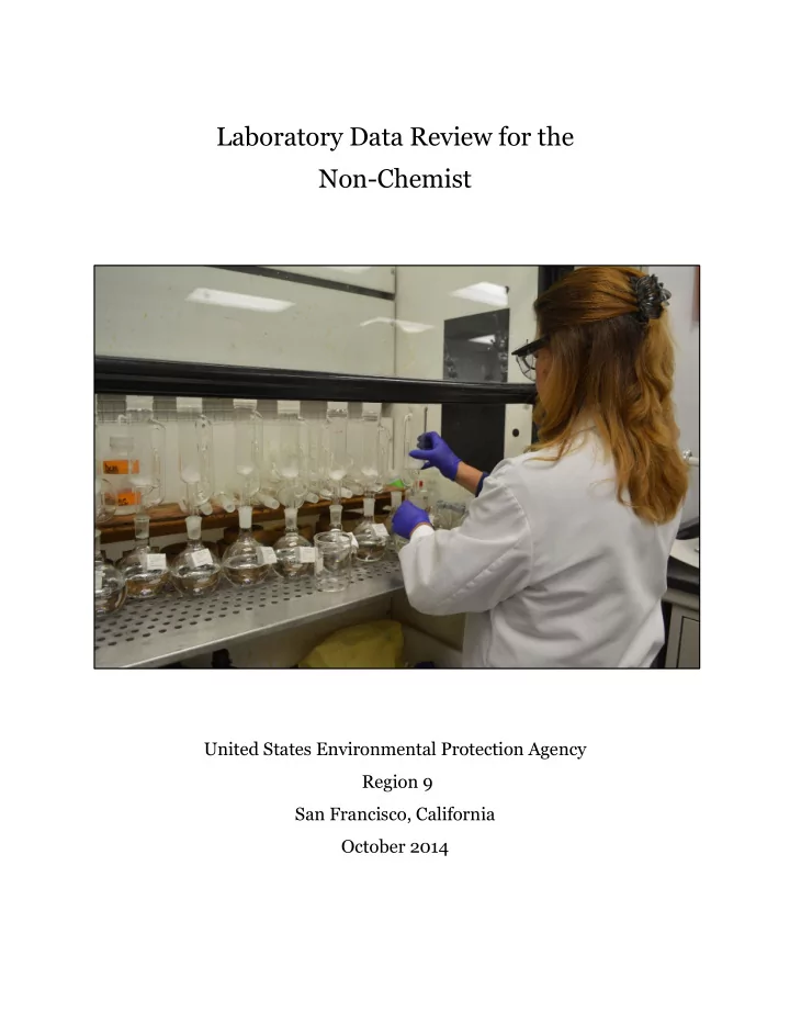
Chemist setting up solvent extraction equipment in a fume hood.

8

3.0 DESK-TOP REVIEW

The desk-top review checklist is shown below, and the following sections explain where the relevant information may be found in the laboratory report.

Desk-Top Review Checklist 3.1

Were problems noted in the case narrative / cover letter?

3.2

Was laboratory accreditation/certification information provided?

3.3

Was laboratory contact information provided?

3.4

Were the date(s) that samples were collected, received, prepared, and analyzed by the laboratory provided?

3.5

Was the correct method used?

3.6

Were all requested analytes reported?

3.7

Were holding times met?

3.8

Were units of measurement reported? (dry/wet weight if applicable)

3.9

Were detection/reporting limits sufficiently low to meet project objectives?

3.10

Were data qualifiers reported and explained?

3.11

Were all surrogate recoveries (organic samples) within allowable limits?

3.12

Was there any contamination in blank samples?

3.13

Were Laboratory Control Sample (LCS) recoveries within allowable limits?

3.14

Were Matrix Spike / Matrix Spike Duplicate or Laboratory Duplicate recoveries within allowable limits?

3.15

Were any interferences noted in the case narrative that could affect the results?

3.16

Were any problems noted on the chain-of-custody form (if provided)?

3.17

Were any problems noted on sample receipt checklist (if provided)?

3.1 Case narrative

The case narrative is typically a short summary statement about the analyses that might include the number and type of samples analyzed. Any significant receipt, analysis, or QA/QC problems should be documented in this section. The case narrative may not actually be called a ‘case narrative’ but is the explanatory text at or near the beginning of the data package. This part of the report should be read carefully, as it helps identify problem samples or problem analyses that could lead to limitations on the use of the data or, in extreme cases, the data’s rejection.

3.2 Laboratory accreditation / certification information

Commercial laboratory’s accreditation / certification information (e.g., state certifications, Department of Defense certification, NELAP certification) is typically provided at or near the beginning of the data package. Note that EPA does not certify any laboratories with the exception of state or tribal facilities that perform drinking water analyses. Certification in and of itself is not a guarantee of good quality data from a laboratory. Accreditation or Certification Inspections usually take place on a yearly or biennial basis and only ensure the laboratory is capable of performing an analysis with a reasonable adherence to established methods at a specific point in time. Accredited laboratories are usually better established and qualified

9

laboratories, but it is the responsibility of project personnel to ensure that the results it receives are of sufficient quality to meet project needs.

3.3 Laboratory contact information

The laboratory should provide a contact name and phone number (and/or email) for questions about its results or the data package it provided. Typically, this information is included at or near the front of the data package or may be at the end of the report.

3.4 Date samples collected, received, prepared, and analyzed

Date information may be found in several different sections of the laboratory report. Frequently, the date(s) that the samples were collected and received at the laboratory is listed in or near the case narrative, while the laboratory preparation/analysis dates are listed within the body of the report.

3.5 Laboratory Method

The method number(s) used in sample preparation and analysis may be listed in a variety of locations, depending on the laboratory. They may be listed in the case narrative, in the header information for each sample, or for each analyte. The method numbers refer to EPA or non-EPA methods, but typically have some code

• r acronym to identify the source of the
• method. Non-EPA method sources

commonly include Standard Methods for the Examination of Water and Wastewater (frequently abbreviated as SM [method number] on laboratory reports); ASTM International (ASTM), which was formerly known as the American Society for Testing and Materials; AOAC (formerly the Association of Official Agricultural Chemists and a good source for pesticide methods); and the National Institute of Occupational Safety and Health (NIOSH) (a source for many health related methods, especially for air analyses). All of the sample preparation and analytical methods listed in the report should be easy to find

• nline using Google or any other search engine. Some methods are subscription-only (e.g.,

ASTM, AOAC, Standard Methods for the Examination of Water and Wastewater), but others are available free of charge (e.g., EPA and NIOSH methods). Availability should be identified on line, and there should be a description of the method, regardless of source, even if it lacks detail. EPA method updates often are listed with a letter designation (e.g., A, B, C) with the later letter indicating the most current update. For example, 8270D is the fourth revision of EPA method 8270, and was preceded by methods 8270C, 8270B, and 8270A. It usually is not necessary to stipulate that the facility use the most current version of a method. Depending on the method, it

Mercury analysis

10

may take some time (up to several years) for an updated version of a method to be widely adopted by commercial laboratories.

3.6 Analytes Reported

Many common EPA analytical methods (e.g., 200.8, 624, 8260, 6010, 8082) are multi-analyte methods that may include several (or dozens) of analytes within a single method. EPA Method 8260 (for volatile organic compounds (VOCs)) currently includes more than 100 analytes, ranging (alphabetically) from acetone to xylene. Few laboratories routinely analyze all 100 compounds, however. For example, the EPA Region 9 Laboratory currently reports 63 analytes using EPA Method 8260. The list of analytes may be reported alphabetically, by CAS (Chemical Abstracts) number, or by retention time on the gas chromatograph (GC) (typically with the most volatile analytes, such as vinyl chloride, reported first). Project managers should ensure that all the analytes necessary for project goals have been

• reported. If obscure/rare analytes are needed, that information should be communicated to the

laboratory prior to sample analysis. Method development, usually performed at an extra cost, should be negotiated in advance. 3.6.1 Analyte Names The same analyte may be reported by different names depending on the laboratory, which can be confusing to novice reviewers. The CAS number is the most definitive means of identifying a chemical, but not all laboratory reports include the CAS number. When in doubt, search for the chemical name online to find synonyms. Some examples of chemical synonyms: methyl ethyl ketone (MEK) = 2 butanone (CAS 78-93-3) methylene chloride = dichloromethane (CAS 75-09-2) perchloroethylene (PCE) = perchloroethene = tetrachloroethylene = tetrachloroethene (CAS 127-18-4) Similar-looking chemical names are not necessarily the same chemical. For example, 1,1-dichloroethene (CAS 75-35-4) is not the same as 1,1-dichloroethane (CAS 75-34-3). 3.6.2 Tentatively Identified Compounds (TICs) Tentatively Identified Compounds (TICs), which may be found in a gas chromatography/mass spectrometry (GC/MS) analysis, may be included in the laboratory

• report. A TIC is a compound which is outside the standard list of analytes in a GC/MS

method, but which is based on a tentative match between the instrument response and the instrument’s computer library. The identification and quantitation of these compounds is

• speculative. TICs should only be used in decision making if they can be confirmed.

3.7 Holding Time

The holding time for a sample is the allowable time between sample collection and sample analysis, and varies by method. Analytes which are somewhat unstable, such as VOCs, have a relatively short hold time (14 days), while the hold time for most metals is six months, since metals are quite stable. Laboratory reports should include the sample collection date/time,

11

sample preparation/extraction date/time, and sample analysis date/time. From these dates and times, report reviewers should be able to determine if the samples were analyzed within the allowable hold time. Information on hold time allowances may be found in SW-846 Chapter 4 Introduction (organic analytes) or Chapter 3 (inorganic analytes). Wastewater holding times can be found in 40 CFR 136 Appendix A. SW-846 is primarily used for solid and hazardous waste analyses, but the equivalent drinking water methods (500 series) and clean water act methods (600 series) have the same holding times. Although holding times appear to be absolutes, some compounds or analytes are more prone to degradation or loss than others, so the laboratory should be consulted if the data do not have regulatory implications. If they do, the holding time must be strictly observed.

3.8 Units of Measurement

Understanding the unit of measurement is key to understanding any laboratory data. Data reported without units are meaningless. The unit of measure may be reported at the top of the page, in a column on the report, in a footnote, or some other location. Report reviewers must always know the reporting units before they can make any decisions about the data. Common reporting units for water samples are micrograms per liter (ug/L) or milligrams per liter (mg/L). Common reporting units for solid samples are micrograms per kilogram (ug/kg) or milligram per kilogram (mg/kg). The units ug/L and ug/kg are often used interchangeably with ‘parts per billion’ or ppb, and mg/L or mg/kg with ‘parts per million’ or ppm. 3.8.1 Wet weight / Dry Weight / ‘As received’ Laboratory reports for soil samples, biota samples, and other solid or semi-solid matrices should also include information about the basis of the measurement, since the reporting units are based on mass (kg) rather than volume (L). Soil or sediment data that will be compared to risk-based values such as EPA Region 9’s Regional Screening Levels (RSLs), California Human Health Screening Levels (CHHSLs), or NOAA Screening Quick Reference Tables (SQRTs) is typically reported as ‘dry weight,’ meaning that the data have been corrected for soil moisture content. Soil or sediment samples that are reported as ‘wet weight’ or ‘as received’ have not had any correction for soil moisture. Fish and other biota samples are typically reported ‘as received,’ which means there has been no correction for the water or oil content of the fish. Fish sample data may also include information about the part of the fish sampled (e.g., fillet, whole fish, or plug from fish tissue).

3.9 Detection / Reporting Limits

Laboratories will report one or more ‘limits,’ including detection limits, reporting limits, quantitation limits, or some other related term. The specific terminology used is not consistent from one laboratory to the next, so reviewers need to carefully examine the laboratory report to ensure that whatever ‘limit’ is used meets project goals. For example, a drinking water sample that is reported as ‘non-detect’ for trichloroethylene (TCE) at a detection limit 10 ug/L would be unusable, because the drinking water standard for TCE is 5 ug/L. A detection limit of 10 ug/L does not provide enough information to determine that the TCE concentration is actually below 5 ug/L. However, the data might be perfectly usable for some other purpose. Non-detects may be reported in a variety of formats: ND in one column, followed by the detection limit in the next

12

column, or even simply ‘ < 1 ug/L’ which means that the analyte was not detected, and the detection limit is 1 ug/L.

3.10 Data Qualifiers

Data qualifiers are laboratory codes that provide comments on the data. An explanation of data qualifiers used by the laboratory should be included in every laboratory report, typically at the end of the report or as footnotes on each page. Data qualifiers vary from laboratory to laboratory, but two fairly universal qualifiers are ‘U’ for non-detect and ‘J’ for estimated value (usually for very low concentration hits). Report reviewers should read and understand the qualifiers to better use the data.

3.11 Surrogate Recoveries

Surrogates are chemicals used in some organic analyses (e.g., VOCs, SVOCs, pesticides/PCBs) that are similar to the target analyte(s) in chemical composition and behavior, but which are not expected to be present in the sample. An example would be the use of fluorinated organic compounds in an analysis which looks for chlorinated and brominated compounds, or isotopically labeled compounds in GC/MS analyses. Surrogates are added to all environmental samples, blanks, and QC samples in the analytical batch during the preparation stage of the

• analysis. Because they are added to all samples, surrogates provide an indicator of performance

that a MS/MSD spike, which is added to only one sample per batch, cannot. Surrogates are used to monitor analytical performance, especially extraction efficiency, purging efficiency (for volatiles), and possible matrix effects. Surrogates are usually not used for inorganic analyses such as metals or nutrients, although occasionally they are used in a few metals methods. Report reviewers should evaluate the percent recovery and allowable range listed for each surrogate compound. Ideally, a surrogate’s recovery should be close to 100%, but there are many reasons that it may be (significantly) less than 100%, and may even be 0% for very high concentration samples where the surrogate was diluted out (this scenario should be noted in the data qualifiers, case narrative, or somewhere else in the laboratory report). The laboratory report will show surrogate recoveries as a percentage, and also the allowable range, which varies by laboratory and by analyte. Allowable surrogate recoveries ideally would be in the range of +/- 30% (i.e., 70 to 130% recovery), but are frequently lower, and potentially much lower for hard- to-analyze compounds. Low (or, less commonly high) surrogate recoveries often trigger a re- extraction and re-analysis by the laboratory. This should be discussed in the case narrative. For some multi-analyte analyses where several different surrogates may be used, some compounds may be within acceptance ranges and some may not. In this scenario, reviewers should discuss with their laboratory what compound results may have been called into question, and whether a reanalysis was conducted.

3.12 Blank contamination

Laboratory reports may contain several types of blank samples that go by a variety of names, but usually include the word ‘blank.’ Blanks are designed to measure cross-contamination in different parts of the sampling and analytical process. An equipment blank is designed to monitor the cleanliness of field equipment. A trip blank (usually only used for VOCs) is designed to measure cross-contamination that may occur during sample handling and transport (e.g., from a broken bottle in the sample ice chest). An instrument blank measures cross-

13

contamination in the analytical instrument. For example, a high concentration sample may cross-contaminate a low concentration sample that follows it. Figure 1 is an illustration of common blank samples, what they are intended to measure, and the potential source of contamination. Equipment blanks are intended to measure contamination from inadequately-cleaned sampling equipment, but can be contaminated in the field or in the

• laboratory. Method blanks, on the other hand, are intended to measure contamination in the

analytical process and can only be contaminated in the laboratory, since they are never in the

• field. A comparison of blank samples can be useful in determining the source of contamination.

For example, if both an equipment blank and a method blank (the two most commonly used blanks) show comparable levels of contamination, the problem would be attributed to the

• laboratory. On the other hand, contamination in the equipment blank, but not the method blank,

would suggest that problems originated in the field. Common field contaminants include equipment decontamination solvents such as hexane and acetone. Common laboratory contaminants include acetone, methylene chloride, and toluene in the volatile fraction (VOCs) and some types

• f phthalates, such as bis (2-ethylhexyl)

phthalate, in the semi-volatile fraction (SVOCs). Phthalates are found in plastic, and plastic is common in laboratories (and in the field). In the absence of any other significant detected analytes, low concentrations (low ppb range) of these common field and laboratory contaminants can usually be ignored.

Dichloromethane (methylene chloride) is a common laboratory contaminant.

Instrument Blank Method Blank Sample Analysis Sample Prep Trip Blank Sample Transport Equipment Blank Field Sampling or Equipment Decontamination Contamination from field or lab Contamination from lab Figure 1 Types of blank samples

14

Some contaminants such as acetone are common laboratory contaminants, but are also organic breakdown products and frequently present at hazardous waste sites. In these cases, determining if a detected analyte is ‘real’ or is an artifact of the sampling/analytical process can be difficult. Comparisons of historical site data and known contaminants at the facility can be useful in determining the source of contamination.

Units MW-1 MW-2 MW-3 Equipment Blank Method Blank Trip Blank hexane ug/L 3 ND ND 12 ND ND chloroform ug/L ND 7 ND 4 ND ND methylene chloride ug/L ND ND 2 ND ND ND

In the example shown above, the equipment blank contains hexane, probably due to inadequate rinsing during equipment decontamination. Sample MW-1, which contains 3 ug/L hexane, is probably an artifact of the inadequate decontamination procedure. The example shown for chloroform, however, is less intuitively obvious. In this case, well MW-2 should be considered non-detect for chloroform, even though the chloroform concentration in well MW-2 is higher than the equipment blank. Chloroform is a disinfection by-product commonly found in tap

• water. Chloroform is frequently found at low concentrations in equipment blank samples if the

equipment did not undergo a final rinse with distilled/deionized water, and MW-2 was probably the first well sampled after the equipment blank was collected. Lastly, the low concentration of methylene chloride in MW-3 may be from cross-contamination in the laboratory (methylene chloride is a common laboratory solvent), even though methylene chloride was not detected in any of the blanks.

3.13 Laboratory Control Sample (LCS)

The Laboratory Control Sample (LCS) is also sometimes called a blank spike (BS) or Laboratory Fortified Blank. An LCS is used to demonstrate laboratory performance. An LCS consists of ultra-pure water or other neutral matrix like laboratory sand, spiked with known concentrations

• f target analytes (if the target analyte list is long, the LCS may contain a subset of the target

analytes). The spiking occurs at the laboratory prior to sample preparation and analysis. The theory behind an LCS is that the laboratory should be able to reliably measure the concentration

• f a target analyte when that analyte is spiked into an interference-free medium.

Laboratory report reviewers should look for a sample labelled ‘LCS’ or ‘BS’ or one called out as a ‘Laboratory Control Sample’ or ‘Blank Spike.’ Data for the LCS/BS usually includes the analyte spike concentration, the analytical result, the percent recovery, and the allowable percent recovery limits. Ideally, the percent recovery will be close to 100%, but some compounds are more reliably recovered than others, so acceptance windows may be defined by the method or the laboratory. Failure to achieve an acceptable recovery for any compound used in an LCS is a major indicator of a laboratory problem. LCS failures are usually caused by problems with either the sample preparation, the analyst, or the analytical instrument. Unacceptable LCS recoveries should trigger a re-preparation and reanalysis of the entire batch associated with the specific LCS. The laboratory should discuss its action in its case narrative. In another situation, a poor matrix spike result, coupled with an acceptable LCS recovery, is a strong indicator that

15

there is a matrix issue with one or more samples. Some laboratories may also perform a LCS/LCSD (Laboratory Control Sample Duplicate) analysis as a means of assessing precision.

3.14 Matrix Spike / Matrix Spike Duplicate (MS/MSD)

A Matrix Spike (MS) sample is an environmental sample (e.g., water, soil) that has been spiked with known concentrations of target analytes. The spiking occurs at the laboratory prior to sample preparation and analysis. A matrix spike is primarily used to assess the matrix effects of a given sample matrix, but it also provides some information on bias. A matrix spike duplicate (MSD) is an intra-laboratory (within the same laboratory) split sample spiked with known concentrations of target analytes. A matrix spike duplicate is used to assess the precision of a method in a given sample matrix. Laboratory report reviewers should look for sample(s) labelled MS and MSD or samples called

• ut as a ‘Matrix Spike’ or ‘Matrix Spike Duplicate.’ Data for the MS/MSD usually includes the
• riginal (source) sample result for the target analyte(s), the spike concentration, the analytical

result, the percent recovery, the percent recovery range limits, and, for the MSD, the Relative Percent Difference (RPD) between the MS and MSD results. Like other laboratory QC results (e.g., LCS, surrogates), the percent recovery ideally should be close to 100%, but may vary considerably from this value. Method and/or laboratory limits should be used to evaluate the acceptability of these recoveries. MS samples are intended to evaluate potential matrix effects, which can impart either a positive or negative bias. Poor recoveries, for example, may indicate that the matrix is suppressing the signal. If this is observed, then surrogate recoveries (for

• rganic analysis, but not inorganic analyses) should also be affected, but LCS results should not.

If LCS results are also poor, this indicates a laboratory problem as discussed previously. Note that MS/MSD samples are usually run on a batch basis, typically 20 samples. If all 20 samples are reasonably homogeneous (e.g., surface water), one could generalize the matrix problem as being pervasive, and factor this into one’s environmental decisions. However, if the 20 samples represent a variety of different matrices (for example, soils of varying organic content or percentage of clay from the same general area), then the MS/MSD results may be of limited value, since only one of the different matrices was spiked. Also, unless specifically requested not to, a laboratory may batch a small sample lot with another small sample lot from a different sample source to make up a batch of 20. In that case, a sample from the other sampler’s collection may be spiked. This would provide no information on possible interferences for your sample set, although laboratory performance with respect to recoveries and precision could still provide useful information. If possible, a request can be made to the laboratory to use one of your samples for spiking purposes (and your sampling team should make sure sufficient sample is provided for three analyses), however, some laboratories charge for two additional analyses if the MS/MSD sample is designated. If the laboratory selects the sample, it is usually done at no additional cost. The laboratory should be consulted on its policies. In some ways, surrogates, which are added to every sample, provide a more useful means of assessing matrix effects and laboratory performance than do MS samples. Finally, if results are from a regular monitoring event such as routine groundwater monitoring, historical data can be consulted to see whether matrix interferences are a recurring problem.

16

3.14.1 Relative Percent Difference (RPD) Calculation Relative Percent Difference (RPD) is calculated the same way for any duplicate pair, such as the MS/MSD, LCS/LCSD, field sample and duplicate, or split samples (duplicate samples analyzed by different laboratories). The RPD is the difference between the results divided by the mean of the results multiplied by 100 to get percent: RPD = Difference between duplicate results Mean of duplicate results x 100 = % RPD example: for field duplicate samples of 136 ug/L and 152 ug/L, the RPD would be: RPD = 152 − 136 144 = 16 144 = 0.11 x 100 = 11 % Note that RPD can be a useful measure of precision, but should be evaluated in context, especially for very low concentration samples. For example, the RPD of duplicate samples that are 3 ug/L and 2 ug/L would be 40% ((3-2)/2.5), which seems high even though the actual analytical results are very close to each other. Ideally, duplicate water samples will have RPDs less than 20% and soil samples less than 30%, but if RPDs exceed this, it doesn’t necessarily mean the data are of poor quality. There are many reasons for high RPDs, including sample heterogeneity or samples with high contaminant

• concentrations. RPD results should be evaluated within the scope of the entire

sampling/analytical program.

3.15 Interferences

The case narrative should note significant analytical interferences and the effect(s) on the data. Interference (primarily matrix interference) is bias that is introduced because something in the sample interferes with the analytical system’s ability to provide an accurate measurement. The interference may be physical (turbidity in storm water could block light transmission in an analysis based on UV absorbance), chemical (a chemical similar to the analyte of interest may react with the analyte of interest that affects the response of the instrument, or spectroscopic (the detector receives an enhanced or suppressed signal due to an emission or an absorbance caused by some other chemical or species in the matrix). Interferences can be positive (more analyte is detected than is present), or negative (less analyte is detected than is present).

17

3.16 Chain of Custody (CoC) Form

The laboratory chain of custody form is the primary means of tracking samples from the field to the laboratory. Also, as the name implies, the chain of custody form documents possession of the samples, typically through signatures of field and laboratory personnel. A copy of the chain

• f custody form may (or may not) be

included in the laboratory report. Key items to review on the CoC are the requested analyses, shipping container temperature upon receipt at the laboratory, date/time of sample collection, and notes/comments on the samples such as strong odors, lack of proper preservation, and broken bottles.

3.17 Laboratory Sample Receipt Checklist

Some laboratories will provide a sample receipt checklist which may be included in the laboratory report and may include some of the same information found on the chain of custody

• form. A sample receipt checklist may include items such as cooler temperature upon receipt at

the laboratory, broken bottles, chemical preservation information, and other details relevant to the project.

Filling out a chain of custody form

18

4.0 SPECIAL TOPICS

4.1 Air / vapor analysis reporting units

Air or soil vapor analyses may be reported in a variety of measurement units, including micrograms per cubic meter (ug/m3), parts per billion volume (ppbV), parts per million volume (ppmV), micrograms per liter (ug/L), or percent (% is typically used for methane). Some laboratories will report data in two different units in different columns on the

• report. Conversion between

units is not intuitive, since ug/ m3 is a weight-to-volume ratio and ppbV is a volume-to- volume ratio. The best approach is to ensure that the laboratory reports the data in the units needed by the data user (typically ug/m3 for risk-based inhalation goals), or, if needed, consult an on-line conversion calculator. Calculators may be found by using the search term: indoor air unit conversion calculator.

4.2 Hazardous Waste Leachability Testing

Under the Resource Conservation and Recovery Act (RCRA), one of the factors that can define a hazardous waste is whether unacceptable levels of specific metals

• r organic chemicals can be leached from it. The

primary USEPA leachability test for hazardous waste (40 CFR Part 261.24) is the Toxicity Characteristic Leaching Procedure (TCLP). In EPA Region 9, the state of California also has a leachability test called the Waste Extraction Test (WET). The leaching test, whether Federal or California, is a sample preparation method, not an analytical method. Samples of soil or waste material are leached using a slightly acidic solution which is designed to simulate leaching that might occur if the waste is buried in a

• landfill. Once the leaching is complete, the leachate (a

liquid) is analyzed by the appropriate analytical method.

Stainless steel air sampling canisters TCLP extracts

19

Comparison of TCLP and WET

TCLP (Federal) WET (California)

20-fold dilution 10-fold dilution acetic acid/buffer extraction citric acid extraction 18 hours extraction 48 hours extraction 7 inorganic compounds 19 inorganic compounds 23 organic compounds 18 organic compounds generally more aggressive than TCLP

TCLP/WET data reporting is often confusing for report reviewers. The 10- or 20-fold dilution means that many analytes can be screened out prior to analysis because the leachable results would not exceed hazardous waste criteria. For example, the TCLP lead (Pb) limit is 5 mg/L. Therefore, if the total concentration of Pb in a waste sample is less than 100 mg/kg, the TCLP test need not be run since the leachable concentration, even if all the Pb were leachable, would not exceed 5 mg/L. In practice, the total Pb concentration is usually significantly higher than 100 mg/kg, thereby resulting in a leachable concentration exceeding the 5 mg/L standard.

4.3 Fish / biota analysis

Fish, plants, and similar materials pose challenges for laboratory analysis, and should be carefully planned with the laboratory before conducted. Data from these materials are typically reported on an ‘as received’ basis (i.e., no correction for water content). Analytical interferences for organic compounds may include the natural oils or fat in the material (especially fish). Analyses can be affected by factors such as whether an entire fish is analyzed or only a fillet, a whole plant or only the leaves, or similar situations. Often a surrogate material is used for laboratory control samples, for example chicken for fish, so reviewers should be aware that LCS results are not necessarily as comparable as they might be for soil or water analyses. Matrix spike results can provide some insight into recoveries for these less routine matrices. Usually metals involve the digestion of the whole sample, so interferences are less of an issue, but can still be found.

4.4 Odd matrices

Environmental laboratories work best with normal environmental matrices such as surface water, groundwater, soil, or air. Odd matrices such as concrete, auto shredder waste, wood, or oily waste will be a challenge to analyze. Likewise, analysis of samples with very high target (or even non-target) contaminant concentrations or high/low pH may result in data with many data

• qualifiers. It may look like ‘unacceptable’ data, but project managers should evaluate the data

within the overall context of the project and pay special attention to QC results.

20

5.0 GLOSSARY

ACCURACY and PRECISION: ACCURACY is the closeness of agreement between an

• bserved value and the true value. PRECISION is a measure of the reproducibility of a value,

without knowledge of the true value. The classic example used to illustrate these terms is a dartboard example: the placement of four darts thrown at a dartboard is considered accurate if all four darts are each close to the bullseye (regardless of their proximity to one another). The placement is considered precise if the darts are all grouped closely together, regardless of their distance from the bullseye. Hence, to be both accurate and precise, the four darts would need to be grouped closely together and be close to the bullseye. ANALYTE: That which is analyzed for. This can be chemical (benzene, chromium), biological (fecal coliform bacteria), mineral (asbestos fibers), or radiological (alpha and beta emissions). BATCH: A group of samples which are processed together. Ideally, all the samples in a batch will be similar enough that matrix QC measurements performed with the batch will be representative of all of the samples in the batch. Most environmental laboratories batch samples in groups of 20. See also Sample Delivery Group. BIAS: A systematic difference between the reported result and the true result. Bias may be introduced through field or laboratory variability and error or due to substances in the sample which interfere with the analytical system’s ability to provide an accurate measurement. Since the true concentration of an analyte in an environmental sample is generally never known, bias is estimated by using surrogates, matrix spikes, laboratory control standards, and other indicators of analytical accuracy. BLANK: See Equipment Blank, Field Blank, Method Blank, Storage Blank, Temperature Blank

• r Trip Blank.

BLANK SPIKE: See Laboratory Control Sample BLIND: A term used to denote various types of QA/QC samples which are submitted to a laboratory for analysis without the laboratory knowing that they are QA/QC samples. Field duplicates are one example of samples that should be sent ‘blind’ to the laboratory. Sample IDs

Not Accurate

• r Precise

Accurate Precise Accurate and Precise

21

for field duplicates should be similar to environmental samples and not identified as duplicates. For example, if the environmental sample is ‘MW-5,’ the field duplicate should not be identified as ‘MW-5 Dupe’ or ‘MW-5D.’ Single or double blind PE samples are another typical blind sample. CALIBRATION: The process of correlating instrument signal response with analyte

• concentration. An instrument must be properly calibrated in order to produce accurate results.

CONTROL LIMITS: Ranges of acceptable results for each type of QC measurement. They may be set up on a project specific basis, or they may be derived internally at a laboratory from historic QC performance data. CONTROL SAMPLE: A quality control sample introduced into a process to monitor the performance of the system. See also: Laboratory Control Sample DATA VALIDATION: The formal, rigorous process by which trained chemists evaluate the quality of laboratory analytical data reports, check for calculation errors and analyte identification errors, and provide information to help the data user determine the usability of the data. DESK-TOP REVIEW: A less-rigorous process which project managers (non-chemists) can use to evaluate the quality of laboratory analytical reports. DETECTION LIMIT: The lowest concentration that can be determined to be statistically different from a blank. DUPLICATE: See Field Duplicate, Matrix Spike Duplicate and Laboratory Duplicate ENVIRONMENTAL SAMPLE: A sample taken un-altered (as much as possible) from the environment (as opposed to a blank, LCS, or other quality control sample). EQUIPMENT BLANK: A sample of ultra-pure water which has been used to rinse decontaminated (i.e., clean) sampling equipment and which is then submitted to the laboratory (usually as a ‘blind’ sample) to assess the effectiveness of the equipment decontamination

• process. An Equipment Blank may also be referred to as a Rinsate Blank.

FIELD: Where environmental samples are collected (‘in the field’). The ‘field’ may be a Superfund hazardous waste site, an NPDES-regulated facility, an office building, a lake, a landfill, or any other location where environmental samples are collected. Rarely, the ‘field’ is an actual field (e.g., meadow, pasture, or paddock). FIELD BLANK: A sample containing ultra-pure water which is collected and processed in exactly the same manner as an equivalent environmental sample (e.g., clean water is poured into a sample container in the same physical location where the environmental samples are collected and is subsequently handled, processed, and analyzed exactly as an equivalent environmental sample). The field blank is used to identify contamination resulting from field conditions. The field blank may also be called a ‘bottle blank,’ and was historically used to document sample bottle cleanliness when sampling bottles were cleaned and re-used. Currently, nearly all

22

environmental sampling projects use sample bottles certified clean by the bottle supplier, so the field blank (bottle blank) is somewhat redundant (and less commonly used today). A less preferable environmental QC sample than an equipment blank, but may be used in cases where an equipment blank is not required (e.g, only disposable equipment is used to collect samples or a situation where samples are collected directly into the sample bottle). FIELD DUPLICATES: Separate and independent environmental samples collected as close together in space and time as possible. These duplicates (usually sent ‘blind’ to the laboratory) are analyzed separately and are useful in documenting the precision of the sampling and analysis

• process. Field duplicates differ from split samples in that they are sent to the same laboratory.

Ideally, a field duplicate is created from a well homogenized environmental sample that is divided in the field. Sometimes the term “Field Replicate” is used for a sample that cannot be split such as a co-located sample used for VOC analyses. Sometimes the term “field replicate” is used interchangeably with field “duplicate.” INSTRUMENT DETECTION LIMIT (IDL): The smallest signal above background noise that an instrument can detect reliably. LABORATORY DUPLICATE: Two portions of the same sample that are prepared and analyzed separately by the laboratory. Also called a Sample Duplicate, the laboratory duplicate is a laboratory (not field) quality control sample that is used to evaluate laboratory precision. Most often used for inorganic analyses. LABORATORY CONTROL SAMPLE (LCS): The laboratory control sample is a known matrix that contains spiked amounts of target compounds or analytes. A laboratory control sample is used to document laboratory performance. An LCS usually consists of ultra-pure water or clean sand that is spiked with known concentrations of the target analytes (if the list of target analytes is long, the LCS may contain a subset of the target analytes). The spiking occurs at the laboratory prior to sample preparation and analysis. The theory behind an LCS is that the laboratory should be able to reliably measure the concentration of a target analyte that is spiked into a “clean” matrix. The LCS may also called a ‘Blank Spike’ or Laboratory Control Standard in laboratory reports. MATRIX: The type of sample (e.g., water, air, sediment, soil, fish tissue). The plural of matrix is matrices. MATRIX INTERFERENCE: Bias introduced because something in the sample interferes with the analytical system’s ability to provide an accurate measurement. The interference may be physical (turbidity in storm water could block light transmission in an analysis based on UV absorbance), chemical (a chemical similar to the analyte of interest may react with the analyte of interest that affects the response of the instrument), or spectroscopic (the detector receives an enhanced or suppressed signal due to an emission or an absorbance caused by some other chemical or species in the matrix). Interferences can be positive (more analyte is detected than is present) or negative (less analyte is detected than is present). MATRIX SPIKE: A measured amount of sample spiked with a known concentration of target

• analytes. The spiking occurs at the laboratory prior to sample preparation and analysis. A

23

matrix spike is used to assess effects of the matrix on analyte concentrations. As such, a MS helps determine the bias of a method in a given sample matrix. MATRIX SPIKE DUPLICATE: Intra-laboratory (within the same laboratory) split samples spiked with identical concentrations of target analytes. The spiking occurs at the laboratory prior to sample preparation and analysis. A matrix spike duplicate is used to assess the precision of a method in a given sample matrix. MSDs are primarily used in organic analyses for semivolatile

• rganic compounds, volatile organic compounds, and pesticides, since these samples often do

not contain naturally occurring chemicals making it difficult to calculate a precision value

• therwise.

METHOD BLANK: An analyte-free matrix which is prepared and processed at the laboratory in exactly the same manner as an equivalent environmental sample (i.e., all reagents are added in the same volumes or proportions as used in sample processing). The method blank is used to document contamination resulting from the analytical process. METHOD DETECTION LIMIT (MDL): The minimum concentration of a substance that can be measured and reported with 99% confidence that the analyte concentration is greater than zero. METHOD QUANTITATION LIMIT (MQL): The minimum concentration of a substance that can be quantified with confidence. Often used interchangeably with Reporting Limit, Quantitation Limit, and Practical Quantitation Limit. PERFORMANCE EVALUATION (PE) SAMPLES: Samples with known concentrations of certain target analytes, and which are submitted ‘blind’ to a laboratory as a check of laboratory

• performance. Laboratories also analyze PE samples as part of the laboratory certification
• process. However, the laboratory is aware that it is a PE sample, and, thus, may put its best

efforts into the analysis. PRACTICAL QUANTITATION LIMIT (PQL): The lowest concentration that can be reliably achieved within specified limits of precision and accuracy during routine laboratory

• perating conditions. The PQL is (by definition in SW-846) 5 to 10 times the Method Detection

Limit (MDL). Often used interchangeably with Method Quantitation Limit, Reporting Limit, and Quantitation Limit. PRECISION: A measure of the reproducibility of a result. This should not be confused with Accuracy, nor with “exacting,” “careful,” or “carefully determined.” The colloquial term, “precise measurement,” is not the same as measuring precision. An analytical system may be very precise (yield the same result no matter how many times the analysis is conducted) but very inaccurate at the same time. See Accuracy. QUALITY ASSURANCE (QA): An integrated system or program of activities involving planning, quality control, quality assessment, reporting and quality improvement to ensure that a product or service meets defined standards of quality with a stated level of confidence. In other words, QA is the overall strategy for obtaining a quality product.

24

QUALITY CONTROL (QC): The system of routine technical activities whose purpose is to measure and control the quality of a product or service so that it meets the needs of users. In

• ther words, QC activities are the tactics which are used to measure and control quality.

QUANTITATION LIMIT (QL): The concentration above which quantitative results can be

• btained with a specified degree of confidence. Often used interchangeably with Method

Quantitation Limit, the Practical Quantitation Limit, and the Reporting Limit. REAGENT BLANK: A blank used to test the integrity of reagents used in the laboratory. For example, a new batch of solvent might be tested for impurities, or distilled or deionized water would be tested to ensure that it is pure. RELATIVE PERCENT DIFFERENCE (RPD): A measure of precision. RPD is calculated the same way for any duplicate pair (e.g., field dupes, MS/MSD, split samples). The relative percent difference (RPD) between duplicate analyses is calculated as: RPD = Difference between duplicate results Mean of duplicate results x 100 = % RPD example: for field duplicate samples of 42 ug/L and 50 ug/L, the RPD would be: RPD = 50 − 42 46 = 8 46 = 0.1739 x 100 = 17 % REPORTING LIMIT (RL): The lower limit at which a laboratory reports data. This limit may have no relationship to the detection limit, and is often project and/or site specific. For example, a facility may say to the laboratory, “My action level is ‘x.’ Don’t report anything below ‘x.’” Data reviewers should carefully evaluate laboratory reports with ‘reporting limits’ rather than detection limits. Often used interchangeably with Quantitation Limit, Practical Quantitation Limit, or Method Quantitation Limit. RINSATE BLANK: See Equipment Blank SAMPLE DELIVERY GROUP (SDG): Typically, a batch of samples numbering 20 or fewer. Twenty is a key number for laboratory QC samples. Field personnel should generally try to collect samples in groups of 20 or fewer (including blanks and field duplicates). Generally, a group of 19 samples (one SDG) is easier for the laboratory to manage than a group of 22 samples (two SDGs). How samples will be batched should be discussed with the laboratory. SPIKE: Known amount of analyte that is introduced purposely into a sample (either an environmental sample or a blank) for the purpose of determining whether or not the analytical system can accurately measure the analyte.

25

SPLIT SAMPLES: Samples taken from the same source and/or location at the same time and sent to two different laboratories to be analyzed independently. They are used to assess inter- laboratory accuracy, inter-laboratory precision, the possibility of large errors by one laboratory

• r the other, or the heterogeneity of the samples.

STANDARD REFERENCE MATERIAL (SRM): An environmental material (soil, sediment, waste) with a known and certified concentration of analyte(s) in it. SRMs are analyzed and used to assess method accuracy on a particular matrix. They are sometimes used in place of Laboratory Control Standards. SRMs are very useful if the SRM is a similar matrix to the types

• f samples being analyzed. Unfortunately, only a limited number of types of SRMs are
• available. Oftentimes the source is the National Institute of Standards and Technology (NIST).

STORAGE BLANK: Analyte-free water placed in the refrigerator or other storage area at the laboratory with the environmental samples. The storage blank is used to evaluate whether or not samples may be cross-contaminating each other in storage, or whether a source of contamination exists in the storage area. SURROGATE: A chemical which is similar to the target analyte(s) in chemical composition and behavior in the analytical process, but which is not expected to be present in the sample. Surrogates are added to most organic (e.g., VOCs, SVOCs, PCBs) environmental samples, blanks, and QC samples in the analytical batch during the preparation stage of analysis. Surrogates are used to monitor the performance of the analytical process. An example would be the use of fluorinated organic compounds in an analysis which looks for chlorinated and brominated compounds. Surrogates may also be called System Monitoring Compounds. TARGET ANALYTE: A chemical that is being looked for in an analysis. TEMPERATURE BLANK: A blank water sample that travels with the shipping container (i.e., ice chest) that is only used to measure temperature – it is not used for chemical analysis. Temperature blank information may be found on the chain-of-custody form, on the laboratory’s sample receipt checklist, or noted in the case narrative. TENTATIVELY IDENTIFIED COMPOUND (TIC): A compound which is outside the standard list of analytes in a GC/MS method, but which is reported based on a tentative match between the instrument response and the instrument’s computer library. The identification and quantitation of these compounds is uncertain. TRIP BLANK: a trip blank is a sample of analyte-free media (water or air) transported from the laboratory to the sampling site and returned to the laboratory unopened. A trip blank is intended to document contamination attributable to shipping or field handling procedures. This type of blank is useful in documenting contamination of volatile organic samples (VOCs), but is not typically used for semi-volatile or non-volatile samples because these are less subject to cross- contamination.

26

6.0 QUALITY CONTROL SUMMARY TABLE

6.1 Blank Contamination

TYPE DEFINITION FREQUENCY PURPOSE CORRECTIVE ACTION(s) to consider Equipment or Rinsate Blank A sample created by rinsing sampling equipment after it has been cleaned. Usually 1:10 or each day Help identify contamination due to decontamination procedures, ambient field conditions, storage conditions, or laboratory problems. Discount (do not correct) positives; fix decon procedures; check method blank; check w/lab; possible resample. Field Blank Sample created by adding distilled or deionized water to a container in field. Used when using dedicated or disposable equipment. Usually 1:10 or each day Help identify contamination due to ambient field conditions, bottles/storage conditions, or laboratory problems. Discount (but don't correct) positives, check bottles, check method blank; check w/lab; possible resample. Trip Blank Volatile free water placed in VOA vial by lab and sent to field with bottles. One per shipping container Identify contamination from transit, bottles,

• r laboratory

conditions. Re-evaluate shipping protocols, check method blank; check w/lab. Reagent Blank Sample generated by laboratory to demonstrate reagents are free of contamination. Whenever new batch of reagents received; not all labs run, few report to clients Identify contamination in common chemicals used in laboratory Laboratory should take action with suppliers; reagents should not be used. Laboratory or Method Blank Sample generated by laboratory and introduced at beginning of sample processing 1:batch or 1:20 samples Identify contamination introduced within laboratory. Discount (but do not correct) positives; check w/lab; redo analysis; resample.

27 (digestion, extraction, etc.). Temperature Blank A VOA vial containing clean water generated by laboratory and sent to field with bottles. 1 per cooler Used by the laboratory to check the temperature of the samples upon arrival at the laboratory. Sample results may be biased low due to losses. Non-detects may be false negative. Note in narrative.

6.2 Accuracy (spikes, performance samples)

TYPE DEFINITION FREQUENCY PURPOSE CORRECTIVE ACTION(s) to consider Field Matrix Spike Known amounts

• f representative

compounds are added to samples in field. Sample submitted blind. This is effectively a PE sample. Uncommon QC sample. If run, once per sampling event. Test laboratory performance and ability to obtain correct results. Check w/lab to assess whether can perform method, look at other QC (lab MS, LCS). Laboratory Matrix Spike (MS) Known amounts

• f an analyte or

representative compounds are added to sample(s) in laboratory. 1:20 or 1:batch Identify whether lab has performed method properly or if sample matrix is introducing a positive or negative bias. Check w/lab; determine whether result due to matrix problem or lab problem (look at LCS results, if OK = matrix; see whether a 2nd sample was prepared and run, if 2nd result

• ut = matrix problem,

if in = lab problem). Make sure not other client’s sample due to batch QC. Monitor future site results for

• pattern. Be aware of

matrix bias in results.

28 Determine if spiked sample representative

• f all samples.

Laboratory Control Sample (LCS) aka: Blank Spike or Laboratory Fortified Blank Known amounts

• f an analyte or

representative compounds are added to a "clean" matrix (lab water or clean sand) in laboratory. 1:20 or 1:batch Identify whether lab has performed method properly. Request lab reanalyze all samples in batch associated with LCS if haven't already; possible resample at lab cost; use results w/caution. Instrument Spike Known amounts

• f an analyte or

representative compounds are injected directly in instrument. As needed when contamination suspected. Determine losses of material due to instrument.

• Nothing. Typically not

reported to client. Post Digestion Spike Metals spike made after digestion

• procedure. Used

in method of standard additions to correct for matrix effects. Usually as needed. Permits calculation of results for metals although a matrix effect exists. Not a QC sample per se, used for quantitation. Surrogate Spike Known amounts

• f organic

compounds, similar in behavior to target analytes, are added to samples before processing. In every sample. Mimic behavior of target compounds. Used to identify either matrix or extraction problems. If all surrogates out, require re-extraction. If some out, look at similarities to targets. Re-extraction is possible option. If sample all gone, may need to resample. Single Blind Performance Evaluation (PE) Sample Known amounts

• f an analyte or
• rganic

compounds provided to lab in a labeled vial or bottle. Once a quarter, once a sample shipment, or not at all. Depends on a number of factors. Check laboratory's ability to perform analysis under optimum conditions. Lab should pass when it knows it is being

• tested. Consider

suspension of work if doesn't pass. At minimum, lab should demonstrate how it will address problem.

29 Double Blind Performance Evaluation (PE) Sample Known amounts

• f an analyte or
• rganic

compounds are provided to lab, but are introduced with samples so lab is not aware of presence. Once a quarter, once a sample shipment, or not at all. Depends on a number of factors. Check laboratory's ability to perform analysis without it’s knowing it is being tested. Consider suspension

• f work for that

analysis if lab doesn't

• pass. At minimum,

lab should demonstrate how it will address problem.

6.3 Precision (replicates)

TYPE DEFINITION FREQUENCY PURPOSE CORRECTIVE ACTION(s) to consider Co- Located Sample Second sample collected at same location but different time (water, air) or at a nearby location (soil, sediment). Sent blind to laboratory. Usually 1:10, may not collect if collecting replicates. Determine heterogeneity of matrix, reproducibility of sample technique and laboratory performance. Expand number of samples or area sampled in future events or

• resample. Check

laboratory duplicates or matrix spike duplicates to make sure looking at field variability, not laboratory. Field Replicate (duplicate) A sample divided into two or more homogeneous parts. 1:10 Determine reproducibility of sub- sampling technique and laboratory/method performance. Check laboratory duplicates or matrix spike duplicates to make sure looking at field variability, not

• laboratory. Check field

sampling procedures. In extreme cases, resample. Matrix Spike Duplicate (MSD) A known amounts

• f an analyte or

representative compounds are added in the laboratory to a second aliquot of the sample used for matrix spike. 1:20 or 1:batch Determine laboratory reproducibility or

• precision. MSD is used

because many samples do not contain organic compounds so no results are available on which to do precision calculations. Check LCSD results. View results with caution and be sensitive to upper and lower range of

• concentrations. Check

whether your sample was used for QC if samples were batched, although using another client’s sample is not as critical as in MS.

30 Laboratory Control Sample Duplicate (LCSD) Known amounts of an analyte or representative compounds are added to a second "clean" matrix (lab water or clean sand) in laboratory. Duplicate of LCS. 1:20 or 1:batch Determine laboratory precision without matrix effects. Reanalysis of all samples in batch. Resample at lab cost. Laboratory Duplicate Second processing and analysis of

• sample. Usually

for general chemistry or metals analyses. 1:20 or 1:batch Determine laboratory precision. Check w/lab. Check LCSD results (may not be available for inorganics). View results with caution and be sensitive to upper and lower range of

• concentrations. Check

whether your sample was used for QC if samples were batched, although using another client’s sample is not as critical as in MS. Field Split A field replicate/duplicate that is sent to a second laboratory. Seldom, usually only if problems develop in previous work. Used as a check on laboratories. Check laboratory QC

• results. Consider PE
• samples. Attempt to

determine which lab

• accurate. Determine

which lab to be kept. Laboratory Split A laboratory created replicate/duplicate that is sent to a second laboratory. Seldom, mainly when problem suspected. Determine inter- laboratory precision. Independent assessment of laboratory problems in primary laboratory. Check laboratory QC

• results. Consider PE
• samples. Attempt to

determine which lab accurate and should be kept.

31

6.4 Sensitivity (detection limits)

TYPE DEFINITION FREQUENCY PURPOSE CORRECTIVE ACTION(s) to consider Method Detection Limit (MDL) Determines lowest concentration

• f an analyte

a laboratory can detect. Usually

• nce a year.

Used to establish the lowest limit of reliable instrument measurement. Compare MDL to action levels or regulatory standard to ensure will be able to make required

• decisions. Consider

alternative methods or laboratory if unable to reach objectives. Quantitation Limit (QL) (Often used interchangeably with Reporting Limit (RL) and Practical Quantitation Limit (PQL)) MDL "bumped" up to a level where lab feels confident all positives are

• real. Usually

a factor of 2 to 10 times

• MDL. For a

PQL, factor is 5 to 10. Calculated value after MDL study. Ensures that the laboratory is reporting

• nly analytes it detects

with confidence. Compare QL to action levels or regulatory standard to ensure will be able to make required decisions. Consider alternative methods or laboratory if unable to reach

• bjectives. Consider

having laboratory report at MDL level for some or all analytes.

32

7.0 CASE STUDIES

The case study section includes pages from actual laboratory reports, with call-out boxes to indicate key information. Site/project/client names and commercial laboratory names have been deleted from the reports. Listed below is explanatory information for each case study, with the main topic listed in parentheses: Case Study 1 (Case narrative): The case narrative may not actually be identified as a “case narrative,” but it is the introductory text in the laboratory report which identifies what type and how many samples were collected, any problems identified with the analysis, and, usually, the field sample ID matched to the laboratory sample ID (most labs assign their own sample ID numbers). Case Study 2 (Sample anomaly form): Some laboratory reports will include a sample anomaly form, which may also be identified as a sample receipt checklist. This form is filled out by the individual who receives the samples at the lab and logs them into the laboratory’s sample tracking system. In this example, the individual receiving the samples at the lab noted that two

• ut of three vials for sample EW-1 were received broken. This is a problem because the standard

sample volume for VOCs is three 40 mL vials. The lab can usually work with two vials, but one vial may not be enough for the analysis, so the analytical result may come back as “sample not analyzed – insufficient volume.” Some of the same information recorded on a sample anomaly form (or sample receipt checklist) may also be recorded on the chain of custody (CoC) form. Case Study 3 (detection summary, reporting limits): To simplify report reviewing, some laboratories will provide a detection summary section in the laboratory report. If provided, the detection summary should be in addition to (not instead of) a detailed laboratory report. This example is interesting because it shows the relationship between contaminant concentrations and reporting limits. Highly contaminated samples need to be diluted to bring the sample within the analytical range of the instrument. The dilutions are then factored into the reporting limit. Case Study 4 (basic information): This EPA Region 9 Laboratory report page highlights some

• f the basic information to review in every data package. Reviewers should note the analytes,

units of measurement, analytical/prep method, data qualifiers, detection/reporting/quantitation limit, and, finally, results. Many labs used internal Standard Operating Procedures (SOPs) that are the laboratory’s version of the applicable method. If so, the SOP number should be

• identified. In this example, the lab is using SOP number 354, which follows EPA Method 524.2.

Case Study 5 (basic information): This laboratory report page highlights some key information to review, including the analytical method number, the date samples were collected and the date received at the lab, the units of measurement, reporting limits, qualifiers, surrogate recoveries, and results. The date sampled and received is important information. Most samples are received at the laboratory within approximately one to three days after sample collection. If there is an excessive delay (e.g., more than four days), additional information may be needed. Late delivery can impact sample preservation (samples will not stay chilled) and will cut into the sample hold

• time. For example, the hold time for unpreserved volatile organic compound (VOCs) is seven
• days. If the samples take four days to arrive at the lab, that significantly cuts into the lab’s

ability to analyze the samples within the required time frame. Also, note the method number is

33

listed as “SW846 8260B.” SW-846 is a compendium of EPA solid waste testing methods. Method 8260B is a test for a long list of volatile organic compounds. Many laboratories would cite this as “EPA 8260B” on their laboratory reports, which is equivalent to “SW846 8260B.” Lastly, note the discussion of alternate chemical names on this laboratory report. The CAS number is unique, and the best way of identifying chemicals in a laboratory report, but not all laboratory reports include the CAS number. Case Study 6 (non-detects, basic information): This laboratory report shows one way of reporting non-detects. A non-detect means that the compound was not detected above the relevant limit. In this report, for example, trans-1,2-dichloroethene was listed not detected above 0.5 ug/L, which is shown in the report as “< 0.50” there are several different ways of reporting non-detects, so reviewers should ensure that they understand the specific non-detect reporting format for the report they are reviewing (see section 3.9 in the main document). The method listed is a variation on Case Study 5, which listed the method as “SW846 8260B.” In case study 6, the method is listed as “SW8260B,” which is just a shortened version of “SW846 8260B.” Case Study 7 (reporting limits, data formatting): This laboratory report lists non-detects as “ND,” and then lists the reporting limit (RL) in the next column. So, for example, the last compound in the first column, 1,2-dichloropropane, is listed as ND with a reporting limit of 1.0 ug/L. This means that 1,2-dichloropropane was not detected above 1.0 ug/L. Compare this non- detect reporting format to Case Study 6 (“<0.50”). This case study also highlights the importance of carefully reviewing the data. At first glance, the detections of tetrachloroethene (12 ug/L) and trichloroethene (38 ug/L) are nearly invisible because they blend in with a long string of NDs. Case Study 8 (basic information, dry weight): Basic information to review in this laboratory report includes analytes, analytical method, reporting limit, qualifiers, surrogate recoveries, and basis of measurement. “Dry weight” values for soil samples are explained in section 3.8.1. Also note how non-detects are reported in comparison to case studies 6 and 7. In this format, non- detects are reported as “ND” followed by the qualifier “U” and then the quantitation limit in the next column. So, for example, most of the non-detects on this data sheet are reported as “ND” “U” and “22” in the result, qualifier, and quantitation limits. This means that the individual Aroclors were not detected above a quantitation limit of 22 ug/kg. In this example, it is possible that Aroclors reported as non-detect are present at less than 22 ug/kg, which is why “non-detect” is not the same as “zero.” Any data reported as non-detect should have a corresponding reporting/quantitation/detection limit to indicate that the result is non-detect above the given

• value. This is also an example of a typical EPA Region 9 Laboratory report. To save paper, EPA

Region 9 uses a small font and wraps information from one page to the next, so it is important for reviewers to carefully review all pages to ensure that they are not missing information and not confusing one sample with the next. For example, the data on this page includes Aroclor results for samples SLB 8, 9, and 10, but the % solids information for SLB 10 wraps to the next page (not included in the case studies). Case Study 9 (surrogates, dilution factor): The PCB samples were relatively high in Aroclor 1260 (listed as 11,000 ug/kg for sample MH24-1B), so the surrogate compounds were diluted

• ut. Because the samples were high in PCBs and therefore diluted (40x), the reporting limit is

raised.

34

Case Study 10 (hold times, surrogates, qualifiers): This case study gives an example of calculating the hold time of a sample (time between sample collection and sample prep/analysis). Case Study 11 (relative percent difference): This case study gives an example of calculating Relative Percent Difference (RPD). RPD is the calculation that is used to compare any pair of identical samples, such as field duplicates, MS/MSD, or split samples. Case Study 12 (laboratory contaminants): This is an example of a detected chemical, acetone, which is likely a laboratory contaminant. Acetone and methylene chloride are solvents that are used extensively in analytical laboratories, but they are also target compounds on the VOC list. Since no other VOCs are detected, the hit of acetone can be disregarded (unless the only/primary constituent of concern at the site is acetone, which is very unlikely). Acetone may (or may not) be present in the associated lab or field blanks. Case Study 13 (lab/field contaminants, TICs): This data sheet from a semi-volatile organic compound (SVOC) analysis is non-detect for all target analytes except bis(2-ethylhexyl)

• phthalate. Bis(2-ethylhexyl) phthalate, a plasticizer, is the most common lab contaminant found

in SVOC analysis. Like the acetone example in Case Study 12, if bis(2-ethylhexyl) phthalate is the only compound detected in the SVOC analysis, it is most likely a lab contaminant. This data sheet also shows TICs, or Tentatively Identified Compounds. TICs are tentative identifications based on a match in the analytical instrument’s computer library. Identification is uncertain; TICs are typically not used for decision-making purposes, although they may prompt follow-up analysis in some cases. In this example, the soil samples were from a wetland environment, and the TICs reported are mostly naturally occurring humic and fulvic acids. Case Study 14 (blanks, surrogates): Blanks (field, trip, method, instrument) should be blank (non-detect for all analytes except the surrogates). Do not confuse ‘blank’ with ‘blank spike,’ (or laboratory control sample) which is a spiked sample that will have detected analytes. This data sheet also calls out surrogates. Surrogates are used for many organic analyses, and, where used, are added to every sample in the batch, including the environmental samples, the blanks, the LCS, and the MS/MSD. Case Study 15 (blank spike): Case study 14 was a blank sample. Case study 15 is a blank spike, which is also called a Laboratory Control Sample (LCS). In a blank spike, there should be results for every spiked compound, and, ideally, the results should be fairly close to 100% of the spiked amount. In this example, the BS recoveries (98 – 106%) are within the control limit of 80% to 120% (i.e., 100% +/- 20%). This data sheet also includes a Blank Spike Duplicate (BSD) and comparison of the BS and BSD results ( as calculated by the Relative Percent Difference or RPD). The BSD results (91 – 102%) are also within the control limits of 80 – 120%, and the RPD is 4% for most analytes, which is well below the maximum RPD of 20%. So, this BS/BSD data is acceptable and should not raise concerns for the reviewer. Case Study 16 (LCS, matrix spike): Like case study 15, case study 16 is another example of an LCS. This case study also includes a portion of the Matrix Spike sample (the data wraps to the next page, which is not included here). The call-out box for the matrix spike sample gives an example of calculating percent recovery. Case Study 17 (air/vapor analysis reporting): A key issue with air or soil vapor reporting is the units of measurement. Unlike water or soil, conversion between air/vapor measurement units

35

is not simple. In Case Study 17, the analytes (BTEX and MTBE) are reported in both units of Vppm (vapor parts per million) and ug/L. Ideally, the air or vapor data will be reported in units needed by the reviewer (typically ug/m3 for risk-based decision making). Online calculators are available to do the conversion if the laboratory report is not in the preferred units. This case study also has the odd term, “Reporting Detection Limit.” Most laboratories use either a “reporting limit” or a “detection limit.” Case Study 18 (soil gas analytical report): Like Case Study 17, this is another example of a vapor data report. In this example, the data is reported in units of ppbv (parts per billion volume) and ug/m3. The same analytes are reported in both units, in separate columns, with the associated reporting limit for that analyte. Case Study 19 (leachability testing): This case study is an example of a data sheet for a Waste Extraction Test (WET), which is the California leachability test. See section 4.2 for more information on leachability testing. Case Study 20 (when to seek help): This case narrative suggests that the samples were very

• contaminated. Interpretation of the data, which has some significant QC concerns, may be

challenging for a novice reviewer. When the laboratory report problems are beyond the scope of this guidance, the reviewer should consider getting technical assistance from their state/tribal quality assurance office, or regional EPA Quality Assurance Office. Alternatively, even with substantial QC problems, the data may still be usable. At this particular site, the data simply confirmed that a part of the site that was suspected of high contamination was in fact highly

• contaminated. Generally, it’s easy to analyze relatively clean samples, but more difficult to

analyze samples that are highly contaminated, so QC problems should be expected.

    

  

            

                             

      

   

 

   



     



     



     



     



     



     

 

     



     



     



     



     



     



     



     



     



 

                                                                                                                      

     

The Case Narrative includes information about the samples (sample ID, sample type, date/time collected) and sample receipt and/or analytical information. SDG = Sample Delivery Group (typically 20 samples or one project if fewer than 20) Laboratory Contact Information

Case Study 1

Page 15 of 15

Report reviewers should read sample receipt checklists and sample anomaly forms (if available). Common problems include broken bottles, samples not properly preserved, missing labels, elevated cooler temperature, and mis- match between bottle labels and the chain-of-custody form. Case Study 2

DETECTIONS SUMMARY

Analyte Result Qualifiers Reporting Limit Units Method Client: Attn: Work Order: Project name: Received:

Client Sample ID

Extraction

MW-13

Benzene 2.6 ug/L EPA 8260B EPA 5030C 2.5 1,1-Dichloroethane 12 ug/L EPA 8260B EPA 5030C 5.0 1,2-Dichloroethane 12 ug/L EPA 8260B EPA 5030C 2.5 1,1-Dichloroethene 320 ug/L EPA 8260B EPA 5030C 5.0 c-1,2-Dichloroethene 22 ug/L EPA 8260B EPA 5030C 5.0 Tetrachloroethene 200 ug/L EPA 8260B EPA 5030C 5.0 1,1,2-Trichloro-1,2,2-Trifluoroethane 65 ug/L EPA 8260B EPA 5030C 50 1,1,2-Trichloroethane 7.3 ug/L EPA 8260B EPA 5030C 5.0 Trichloroethene 1700 ug/L EPA 8260B EPA 5030C 20 Vinyl Chloride 2.6 ug/L EPA 8260B EPA 5030C 2.5

IA-1

1,1-Dichloroethene 1.6 ug/L EPA 8260B EPA 5030C 1.0 Tetrachloroethene 2.9 ug/L EPA 8260B EPA 5030C 1.0 Trichloroethene 3.7 ug/L EPA 8260B EPA 5030C 1.0

MW-12

1,1-Dichloroethane 3.8 ug/L EPA 8260B EPA 5030C 2.0 1,2-Dichloroethane 2.9 ug/L EPA 8260B EPA 5030C 1.0 1,1-Dichloroethene 81 ug/L EPA 8260B EPA 5030C 2.0 c-1,2-Dichloroethene 83 ug/L EPA 8260B EPA 5030C 2.0 Tetrachloroethene 23 ug/L EPA 8260B EPA 5030C 2.0 Trichloroethene 400 ug/L EPA 8260B EPA 5030C 2.0

MW-10

1,1-Dichloroethene 4600 ug/L EPA 8260B EPA 5030C 1000 Tetrachloroethene 6800 ug/L EPA 8260B EPA 5030C 1000 Trichloroethene 120000 ug/L EPA 8260B EPA 5030C 1000

DUP 1

1,1-Dichloroethene 4800 ug/L EPA 8260B EPA 5030C 1000 c-1,2-Dichloroethene 1000 ug/L EPA 8260B EPA 5030C 1000 Tetrachloroethene 7000 ug/L EPA 8260B EPA 5030C 1000 Trichloroethene 120000 ug/L EPA 8260B EPA 5030C 1000

Subcontracted analyses, if any, are not included in this summary. *MDL is shown. Note that reporting limits vary. Higher concentration samples are diluted to bring the sample within the range

• f the instrument, so

the reporting limit is raised. Some laboratories provide a summary

• f detections. If

provided, this should be in addition to (not instead of) more detailed information. Case Study 3

    

  

            

                           

           

 

  

       

                                                                                                                                                                                                                                                                                                                                                           

   

     

EPA Method and lab’s Standard Operating Procedure (SOP) for that method. Units of Measurement Lab ID and Sample ID. Most labs assign their

• wn sample ID numbers.

Lab reports should include both the lab and field sample IDs. Laboratory Contact Info Read and understand data qualifiers. Data qualifiers are usually found at the front or back of the data package

• r as footnotes.

Long compound lists may be

• rganized alphabetically,

by retention time on the GC column, by CAS (Chemical Abstracts Service) number,

• r by some other method.

Reviewers should ensure that all needed analytes are reported.

Case Study 4

Report of Analysis

Page 2 of 3 Client Sample ID: MM27-GW-15 Lab Sample ID: C20014-7 Date Sampled: 01/24/12 Matrix: AQ - Ground Water Date Received: 01/25/12 Method: SW846 8260B Percent Solids: n/a Project: VOA 8260 List CAS No. Compound Result RL MDL Units Q 156-60-5 trans-1,2-Dichloroethylene 1.7 1.0 0.20 ug/l 10061-02-6 trans-1,3-Dichloropropene ND 1.0 0.30 ug/l 100-41-4 Ethylbenzene ND 1.0 0.20 ug/l 637-92-3 Ethyl Tert Butyl Ether ND 2.0 0.22 ug/l 591-78-6 2-Hexanone ND 10 2.0 ug/l 87-68-3 Hexachlorobutadiene ND 2.0 0.20 ug/l 98-82-8 Isopropylbenzene ND 1.0 0.20 ug/l 99-87-6 p-Isopropyltoluene ND 2.0 0.20 ug/l 108-10-1 4-Methyl-2-pentanone ND 10 1.0 ug/l 74-83-9 Methyl bromide ND 2.0 0.20 ug/l 74-87-3 Methyl chloride ND 1.0 0.20 ug/l 74-95-3 Methylene bromide ND 1.0 0.20 ug/l 75-09-2 Methylene chloride ND 10 2.0 ug/l 78-93-3 Methyl ethyl ketone a ND 10 2.0 ug/l 1634-04-4 Methyl Tert Butyl Ether 0.25 1.0 0.20 ug/l J 91-20-3 Naphthalene ND 5.0 0.50 ug/l 103-65-1 n-Propylbenzene ND 2.0 0.20 ug/l 100-42-5 Styrene ND 1.0 0.20 ug/l 994-05-8 Tert-Amyl Methyl Ether ND 2.0 0.40 ug/l 75-65-0 Tert-Butyl Alcohol ND 10 2.4 ug/l 630-20-6 1,1,1,2-Tetrachloroethane ND 1.0 0.30 ug/l 71-55-6 1,1,1-Trichloroethane ND 1.0 0.20 ug/l 79-34-5 1,1,2,2-Tetrachloroethane ND 1.0 0.20 ug/l 79-00-5 1,1,2-Trichloroethane 15.8 1.0 0.22 ug/l 87-61-6 1,2,3-Trichlorobenzene ND 2.0 0.20 ug/l 96-18-4 1,2,3-Trichloropropane ND 2.0 0.20 ug/l 120-82-1 1,2,4-Trichlorobenzene ND 2.0 0.20 ug/l 95-63-6 1,2,4-Trimethylbenzene a ND 2.0 0.20 ug/l 108-67-8 1,3,5-Trimethylbenzene ND 2.0 0.20 ug/l 127-18-4 Tetrachloroethylene 2.0 1.0 0.54 ug/l 108-88-3 Toluene ND 1.0 0.20 ug/l 79-01-6 Trichloroethylene 21.9 1.0 0.20 ug/l 75-69-4 Trichlorofluoromethane ND 1.0 0.20 ug/l 75-01-4 Vinyl chloride 0.49 1.0 0.20 ug/l J 1330-20-7 Xylene (total) ND 2.0 0.46 ug/l CAS No. Surrogate Recoveries Run# 1 Run# 2 Limits 1868-53-7 Dibromofluoromethane 102% 60-130% 2037-26-5 Toluene-D8 95% 60-130% ND = Not detected MDL - Method Detection Limit J = Indicates an estimated value RL = Reporting Limit B = Indicates analyte found in associated method blank E = Indicates value exceeds calibration range N = Indicates presumptive evidence of a compound

24 of 34

2

2.7 Method Qualifiers Units of Measurement Results Reporting limits vary depending on the water solubility of the compound, contaminant concentrations, and other factors. Water- soluble compounds such as 2-hexanone, MEK, and TBA have higher reporting limits than less water soluble compounds. Date Sampled and Date Received (at lab) Surrogate Recovery % and Allowable Limit Range Footnotes The same chemical may have different names. Examples: 4-methyl-2-pentanone = MIBK methylene chloride = dichloromethane methyl ethyl ketone (MEK) = 2-butanone Alternate names are easily found

• nline.

The CAS number is more definitive than the name of the compound (see naming discussion lower right)

Case Study 5

Method Dilution Factor Units of Measurement Non Detect. < 0.50 means that the compound was not detected above the detection/reporting limit of 0.50 ug/L Reporting

• r Detection

Limit Date Sampled and Date Analyzed Surrogate Recovery % and Allowable Limit Range Footnotes

Case Study 6

Analytical Report

02/01/11 Date Received: Work Order No: EPA 5030C Preparation: EPA 8260B Method: Project: Page 3 of 19

Lab Sample Number Date/Time Collected Date Prepared Date/Time Analyzed QC Batch ID Client Sample Number Matrix

Units: ug/L

Instrument 01/31/11 02/02/11 02/02/11 Aqueous 110202L01 D2-B1 11-02-0061-3-A GC/MS S 16:09 11:36 Parameter Result RL DF Qual Parameter RL Result DF Qual Acetone 50 1 ND 1,3-Dichloropropane 1.0 1 ND Benzene 0.50 1 ND 2,2-Dichloropropane 1.0 1 ND Bromobenzene 1.0 1 ND 1,1-Dichloropropene 1.0 1 ND Bromochloromethane 1.0 1 ND c-1,3-Dichloropropene 0.50 1 ND Bromodichloromethane 1.0 1 ND t-1,3-Dichloropropene 0.50 1 ND Bromoform 1.0 1 ND Ethylbenzene 1.0 1 ND Bromomethane 10 1 ND 2-Hexanone 10 1 ND 2-Butanone 10 1 ND Isopropylbenzene 1.0 1 ND n-Butylbenzene 1.0 1 ND p-Isopropyltoluene 1.0 1 ND sec-Butylbenzene 1.0 1 ND Methylene Chloride 10 1 ND tert-Butylbenzene 1.0 1 ND 4-Methyl-2-Pentanone 10 1 ND Carbon Disulfide 10 1 ND Naphthalene 10 1 ND Carbon Tetrachloride 0.50 1 ND n-Propylbenzene 1.0 1 ND Chlorobenzene 1.0 1 ND Styrene 1.0 1 ND Chloroethane 5.0 1 ND 1,1,1,2-Tetrachloroethane 1.0 1 ND Chloroform 1.0 1 ND 1,1,2,2-Tetrachloroethane 1.0 1 ND Chloromethane 10 1 ND Tetrachloroethene 1.0 1 12 2-Chlorotoluene 1.0 1 ND Toluene 1.0 1 ND 4-Chlorotoluene 1.0 1 ND 1,2,3-Trichlorobenzene 1.0 1 ND Dibromochloromethane 1.0 1 ND 1,2,4-Trichlorobenzene 1.0 1 ND 1,2-Dibromo-3-Chloropropane 5.0 1 ND 1,1,1-Trichloroethane 1.0 1 ND 1,2-Dibromoethane 1.0 1 ND 1,1,2-Trichloro-1,2,2-Trifluoroethane 10 1 ND Dibromomethane 1.0 1 ND 1,1,2-Trichloroethane 1.0 1 ND 1,2-Dichlorobenzene 1.0 1 ND Trichloroethene 1.0 1 38 1,3-Dichlorobenzene 1.0 1 ND Trichlorofluoromethane 10 1 ND 1,4-Dichlorobenzene 1.0 1 ND 1,2,3-Trichloropropane 5.0 1 ND Dichlorodifluoromethane 1.0 1 ND 1,2,4-Trimethylbenzene 1.0 1 ND 1,1-Dichloroethane 1.0 1 ND 1,3,5-Trimethylbenzene 1.0 1 ND 1,2-Dichloroethane 0.50 1 ND Vinyl Acetate 10 1 ND 1,1-Dichloroethene 1.0 1 ND Vinyl Chloride 0.50 1 ND c-1,2-Dichloroethene 1.0 1 4.2 p/m-Xylene 1.0 1 ND t-1,2-Dichloroethene 1.0 1 ND

• -Xylene

1.0 1 ND 1,2-Dichloropropane 1.0 1 ND Methyl-t-Butyl Ether (MTBE) 1.0 1 ND Surrogates: REC (%) Control Limits Qual Surrogates: REC (%) Control Limits Qual Dibromofluoromethane 102 80-126 1,2-Dichloroethane-d4 103 80-134 Toluene-d8 103 80-120 1,4-Bromofluorobenzene 105 80-120

RL - Reporting Limit , DF - Dilution Factor , Qual - Qualifiers

Preparation and analytical methods Reporting limits vary by analyte even in relatively clean samples. Highly water-soluble compounds, such as acetone and 2-butanone, typically have higher reporting limits. Surrogate Recovery % and Allowable Limit Range If detected analytes are not indicated in bold type or otherwise highlighted, it’s easy to miss important data in a sea of non-detects.

Case Study 7

    

  

            

                             

           

 

  

       

                                                                                

       

                                                                                                                                  

       

                                                                                                                         

   

     

Surrogate Recovery % and Allowable Limit Range Qualifiers: most labs use “U” for “non-detect” The method and the lab’s Standard Operating Procedure (SOP) number for that method The lab uses the % solids content to calculate the soil moisture content, and then transform the ‘wet’ analytical results to ‘dry’ weight values. Although uncommon, sometimes pages are missing from a lab

• report. Check to

ensure that all pages are included. Results Units and basis (dry weight). All analytes reported? The EPA R9 Lab reports nine Aroclors, but many labs only report six or seven Aroclors (Aroclors 1248, 1254, and 1260 are the most common). Ensure that all needed analytes are reported. Case Study 8

Polychlorinated Biphenyls (PCBs)

Lab #: Location: Client: Prep: EPA 3550B Project: Analysis: EPA 8082 Matrix: Soil Sampled: 06/25/13 Units: ug/Kg Received: 06/25/13 Basis: as received Prepared: 06/27/13 Batch#: 200169 Field ID: MH24-1A Diln Fac: 40.00 Type: SAMPLE Analyzed: 06/30/13 Lab ID: 246462-001 Analyte Result RL Aroclor-1016 ND 270 Aroclor-1221 ND 540 Aroclor-1232 ND 270 Aroclor-1242 ND 270 Aroclor-1248 ND 270 Aroclor-1254 ND 270 Aroclor-1260 17,000 270 Surrogate %REC Limits TCMX DO 66-142 Decachlorobiphenyl DO 43-139 Field ID: MH24-1B Diln Fac: 40.00 Type: SAMPLE Analyzed: 06/30/13 Lab ID: 246462-002 Analyte Result RL Aroclor-1016 ND 270 Aroclor-1221 ND 530 Aroclor-1232 ND 270 Aroclor-1242 ND 270 Aroclor-1248 ND 270 Aroclor-1254 ND 270 Aroclor-1260 11,000 270 Surrogate %REC Limits TCMX DO 66-142 Decachlorobiphenyl DO 43-139 DO= Diluted Out ND= Not Detected RL= Reporting Limit

Page 1 of 2 2.1

Surrogate Recovery % and allowable limit range. The surrogate was diluted out due to the high concentration

• f PCBs in the sample

Reporting Limit is raised due to dilutions needed because the sample had high PCBs Units (ug/Kg, or ppb) and “basis.” In this case, the basis is “as received,” which is the same as “wet weight.” Dry weight values (i.e., data corrected for soil moisture content) are needed for most risk- based soil or sediment data evaluations, so reviewers should always check to see if soil/sediment data is reported as wet weight or dry weight. Preparation and analysis methods. Soxhlet extraction (EPA Method 3540) is needed for some PCB analysis, so data reviewers should check that the correct method was used. Diln Fac = Dilution Factor (40x) Case Study 9



                     



         



                                                                                                                                                          



                                                                                                      

 





 



“J qualified” is an estimated value, usually for a result that is above the method detection limit (MDL) but below the reporting limit (RL) Check hold times. The hold time is the time between sample collection and sample analysis. In this example, the hold time was 9 days (9/22/09 to 10/01/09), which is within the allowable hold time of 14 days for EPA Method 8260. Surrogate Recovery % Surrogates and allowable recovery range

Case Study 10

    

  

            

                             

           

 

  

       

                                                                                

       

                                                                                                                                  

       

                                                                                                                         

   

     

SLB9 and SLB10 were field duplicate samples that were submitted “blind” to the laboratory (i.e., not identified as field duplicate samples). Duplicate samples are evaluated by calculating the Relative Percent Difference (RPD): RPD = difference between duplicate results mean of duplicate results So, for Aroclor1254 for the SLB 9 & 10 pair: 150 - 120 30 135 135 = = 0.22 = 22%

Case Study 11

Purgeable Organics by GC/MS

Lab #: Client: Prep: EPA 5030B Project#: Field ID: CR COMP H (1-4) Diln Fac: 0.9823 Lab ID: 254695-008 Batch#: 209215 Matrix: Soil Sampled: 03/19/14 Units: ug/Kg Received: 03/19/14 Basis: as received Analyzed: 03/21/14 Analyte Result RL Freon 12 ND 9.8 Chloromethane ND 9.8 Vinyl Chloride ND 9.8 Bromomethane ND 9.8 Chloroethane ND 9.8 Trichlorofluoromethane ND 4.9 Acetone 39 20 Freon 113 ND 4.9 1,1-Dichloroethene ND 4.9 Methylene Chloride ND 20 Carbon Disulfide ND 4.9 MTBE ND 4.9 trans-1,2-Dichloroethene ND 4.9 Vinyl Acetate ND 49 1,1-Dichloroethane ND 4.9 2-Butanone ND 9.8 cis-1,2-Dichloroethene ND 4.9 2,2-Dichloropropane ND 4.9 Chloroform ND 4.9 Bromochloromethane ND 4.9 1,1,1-Trichloroethane ND 4.9 1,1-Dichloropropene ND 4.9 Carbon Tetrachloride ND 4.9 1,2-Dichloroethane ND 4.9 Benzene ND 4.9 Trichloroethene ND 4.9 1,2-Dichloropropane ND 4.9 Bromodichloromethane ND 4.9 Dibromomethane ND 4.9 4-Methyl-2-Pentanone ND 9.8 cis-1,3-Dichloropropene ND 4.9 Toluene ND 4.9 trans-1,3-Dichloropropene ND 4.9 1,1,2-Trichloroethane ND 4.9 2-Hexanone ND 9.8 1,3-Dichloropropane ND 4.9 Tetrachloroethene ND 4.9 Dibromochloromethane ND 4.9 1,2-Dibromoethane ND 4.9 Chlorobenzene ND 4.9 1,1,1,2-Tetrachloroethane ND 4.9 Ethylbenzene ND 4.9 m,p-Xylenes ND 4.9

• -Xylene ND 4.9

Styrene ND 4.9 Bromoform ND 4.9 Isopropylbenzene ND 4.9 1,1,2,2-Tetrachloroethane ND 4.9 1,2,3-Trichloropropane ND 4.9 Propylbenzene ND 4.9 Bromobenzene ND 4.9 1,3,5-Trimethylbenzene ND 4.9 2-Chlorotoluene ND 4.9 *= Value outside of QC limits; see narrative ND= Not Detected RL= Reporting Limit

Page 1 of 2 22.0

Acetone and methylene chloride are two common laboratory

• contaminants. In the absence of

any other target VOCs, low concentrations of acetone or methylene chloride can usually be ignored. Similar concentrations may (or may not) be found in the blank samples. “as received” = “wet weight” If dry weight values are needed (typically for comparison to risk-based concentrations), the lab must also measure percent solids and correct the analytical results for moisture

• content. Dry weight must be requested

before the samples are analyzed.

Case Study 12

    

  

            

                           

           

 

  

       

                                                                                                                                                                                                                                                                                                                                                                                                                                       

   

     

Read and understand data

• qualifiers. In this case, the

qualifiers indicate that the compound was not detected (U), the value is estimated (J), the MS/MSD did not meet recovery criteria (Q4), and the samples were received at the lab above the ideal temperature (A2). Phthalates (especially bis (2 ethylhexyl) phthalate) are found in plastic and are the most common laboratory contaminant found in semi-volatile

• rganic compound (SVOC)

analyses. TICs are Tentatively Identified Compounds. Although it may seem that this sample is significantly contaminated, these TICs are mainly humic and fulvic acids found naturally in this wetland environment.

Case Study 13

    

  

            

                             

 

 

                                                                                                                                                                                                                                                                                      

   

     

Blank samples are used as a check of cross- contamination in the field or lab depending on the type of blank sample. Surrogates are run on every organic sample, including the environmental samples, the blanks, the LCS, MS, and MSD samples. Case Study 14

Batch QC Report California Title 22 Metals

Lab #: Location: Client: Prep: EPA 3050B Project#: Analysis: EPA 6010B Matrix: Soil Batch#: 209213 Units: mg/Kg Prepared: 03/21/14 Diln Fac: 1.000 Analyzed: 03/21/14 Type: BS Lab ID: QC732739 Analyte Spiked Result %REC Limits Antimony 100.0 98.76 99 80-120 Arsenic 50.00 51.26 103 80-120 Barium 100.0 100.1 100 80-120 Beryllium 2.500 2.654 106 80-120 Cadmium 10.00 10.16 102 80-120 Chromium 100.0 100.2 100 80-120 Cobalt 25.00 25.30 101 80-120 Copper 12.50 12.44 100 80-120 Lead 100.0 98.40 98 80-120 Molybdenum 20.00 20.16 101 80-120 Nickel 25.00 24.87 99 80-120 Selenium 50.00 49.75 99 80-120 Silver 10.00 9.495 95 80-120 Thallium 50.00 49.81 100 80-120 Vanadium 25.00 25.02 100 80-120 Zinc 25.00 25.37 101 80-120 Type: BSD Lab ID: QC732740 Analyte Spiked Result %REC Limits RPD Lim Antimony 100.0 95.46 95 80-120 3 20 Arsenic 50.00 49.30 99 80-120 4 20 Barium 100.0 95.72 96 80-120 4 20 Beryllium 2.500 2.551 102 80-120 4 20 Cadmium 10.00 9.798 98 80-120 4 20 Chromium 100.0 96.17 96 80-120 4 20 Cobalt 25.00 24.23 97 80-120 4 20 Copper 12.50 11.91 95 80-120 4 20 Lead 100.0 94.17 94 80-120 4 20 Molybdenum 20.00 19.40 97 80-120 4 20 Nickel 25.00 23.91 96 80-120 4 20 Selenium 50.00 47.63 95 80-120 4 20 Silver 10.00 9.111 91 80-120 4 20 Thallium 50.00 48.00 96 80-120 4 20 Vanadium 25.00 23.98 96 80-120 4 20 Zinc 25.00 24.37 97 80-120 4 20 RPD= Relative Percent Difference

Page 1 of 1 13.0

Blank Spike (BS) is the same as LCS (Laboratory Control Sample) Blank Spike Duplicate

(Laboratory Control Sample Duplicate)

The ideal % recovery is 100% but the allowable limit in this example is 100% plus or minus 20% (i.e. 80% to 120%) Relative Percent Difference between the BS and BSD result and the allowable maximum RPD. Case Study 15

    

  

            

                           

 

 

                                                                                                                                                                                                                                                                                                                                                                    

   

     

Check Matrix Spike recovery. For this analyte, 5 ug/L was spiked and 7.29 ug/L was detected, resulting in a recovery of 146% 7.29 / 5.00 = 1.458 x 100 = 146% Do not confuse results from LCS and MS/MSD samples with environmental samples. LCS and MS/MSD samples are spiked with analytes, so there should be a positive result. For this analyte, 5 ug/L was spiked and 6.12 ug/L was detected, but the original sample (the “source”) had 0.78 ug/L, which results in a recovery of 106% 6.12 / (5.00 + 0.78) 6.12 / 5.78 = 1.06 x 100 = 106% (lab report shows 107% for technical reasons beyond the scope of this training) Case Study 16

Method Results “Reporting Detection Limit” Date Analyzed and Analyst Footnotes Dilution Factor Units of Measurement: Air/vapor samples may be reported as ug/L, ppmV, ppbV, mg/m3, or ug/m3. Report reviewers must ensure that they understand the units reported and that they are adequate for project goals. In this example, the same information is reported in both Vppm and ug/L..

Case Study 17

Client Sample ID: SVE-04-SG-17 Lab ID#: 0811421-01A MODIFIED EPA METHOD TO-15 GC/MS FULL SCAN

7120208

File Name:

• Dil. Factor:

17.3 Date of Collection: 11/17/08 Date of Analysis: 12/2/08 03:45 PM (uG/m3) (uG/m3) (ppbv) (ppbv) Compound Amount

• Rpt. Limit

Amount

• Rpt. Limit

8.6 20 47 110 1,1,2-Trichloroethane 8.6 2500 59 17000 Tetrachloroethene 35 Not Detected 140 Not Detected 2-Hexanone 8.6 Not Detected 74 Not Detected Dibromochloromethane 8.6 Not Detected 66 Not Detected 1,2-Dibromoethane (E DB) 8.6 Not Detected 40 Not Detected Chlorobenzene 8.6 Not Detected 38 Not Detected E thyl Benzene 8.6 10 38 45 m,p-Xylene 8.6 Not Detected 38 Not Detected

• -Xylene

8.6 Not Detected 37 Not Detected S tyrene 8.6 Not Detected 89 Not Detected Bromoform 8.6 Not Detected 42 Not Detected Cumene 8.6 Not Detected 59 Not Detected 1,1,2,2-Tetrachloroethane 8.6 Not Detected 42 Not Detected Propylbenzene 8.6 Not Detected 42 Not Detected 4-E thyltoluene 8.6 Not Detected 42 Not Detected 1,3,5-Trimethylbenzene 8.6 Not Detected 42 Not Detected 1,2,4-Trimethylbenzene 8.6 Not Detected 52 Not Detected 1,3-Dichlorobenzene 8.6 Not Detected 52 Not Detected 1,4-Dichlorobenzene 8.6 Not Detected 45 Not Detected alpha-Chlorotoluene 8.6 Not Detected 52 Not Detected 1,2-Dichlorobenzene 35 Not Detected 260 Not Detected 1,2,4-Trichlorobenzene 35 Not Detected 370 Not Detected Hexachlorobutadiene Container Type: 1 Liter Summa Canister Limits %Recovery Surrogates Method 99 70-130 Toluene-d8 97 70-130 1,2-Dichloroethane-d4 100 70-130 4-Bromofl uorobenzene

This soil gas report helpfully lists analytes in units of both ppbv and ug/m3, which are two common reporting units for soil gas. Air and soil gas unit conversions (ppbv, ug/m3, ug/L) are very different than water (ug/L, mg/L) or soil (ug/kg, mg/kg) unit conversions.

Soil Gas Analytical Report

Case Study 18

Lab #: Location: Client: Prep: WET Project#: Analysis: EPA 6010B Analyte: Lead Sampled: 03/19/14 Matrix: WET Leachate Received: 03/19/14 Units: ug/L Prepared: 03/30/14 Diln Fac: 10.00 Analyzed: 03/31/14 Batch#: 209539 Field ID Type Lab ID Result RL CR COMP C (1-4) SAMPLE 254695-003 6,700 250 CR COMP E (1-4) SAMPLE 254695-005 22,000 250 CR COMP F (1-4) SAMPLE 254695-006 2,400 250 CR COMP G (1-4) SAMPLE 254695-007 1,800 250 CR COMP H (1-4) SAMPLE 254695-008 ND 250 BLANK QC734038 ND 250

Lead

ND= Not Detected RL= Reporting Limit

The California Waste Extraction Test (WET) is the test used to determine compliance with California’s Soluble Threshold Limit Concentration (STLC). WET is similar to, but more aggressive than, the Federal (EPA) TCLP test. Measurement units are important for data interpretation. In this example, the leachable metals data (WET) is reported as ug/L, but the California Title 22 hazardous waste limits are listed in mg/L. Two of these samples exceed the Title 22 leachable lead (Pb) limit of 5,000 ug/L (5 mg/L): 6,700 ug/L = 6.7 mg/L 22,000 ug/L = 22 mg/L WET (or TCLP) is an extraction

• method. The extract

(leachate) is then analyzed (in this example, by EPA Method 6010B for metals). Case Study 19

CASE NARRATIVE Laboratory number: Client: Project: Location: Request Date: 03/19/14 Samples Received: 03/19/14

This data package contains sample and QC results for nine soil samples, requested for the above referenced project on 03/19/14. The samples were received cold and intact. TPH-Purgeables and/or BTXE by GC (EPA 8015B): No analytical problems were encountered. TPH-Extractables by GC (EPA 8015B): Many samples were diluted due to the dark and viscous nature of the sample

• extracts. No other analytical problems were encountered.

Volatile Organics by GC/MS (EPA 8260B): Low surrogate recovery was observed for dibromofluoromethane in CR COMP H (1-4) (lab # 254695-008). No other analytical problems were encountered. Semivolatile Organics by GC/MS (EPA 8270C): Low recoveries were observed for a number of analytes in the MS/MSD of IR68 COMP1A,B,C,D (lab # 254692-001); the LCS was within limits, and the associated RPDs were within limits. Low surrogate recoveries were observed for 2,4,6-tribromophenol in CR COMP H (1-4) (lab # 254695-008) and the MS/MSD

• f IR68 COMP1A,B,C,D (lab # 254692-001). Low surrogate recoveries were
• bserved for 2-fluorophenol in the MS/MSD of IR68 COMP1A,B,C,D (lab #

254692-001). No other analytical problems were encountered. PCBs (EPA 8082): All samples underwent sulfuric acid cleanup using EPA Method 3665A. All samples underwent sulfur cleanup using the copper option in EPA Method 3660B. No analytical problems were encountered. Metals (EPA 6010B and EPA 7471A) Soil: High recoveries were observed for copper and zinc in the MS/MSD for batch 209213; the parent sample was not a project sample, the BS/BSD were within limits, and the associated RPDs were within limits. High recoveries were

• bserved for mercury in the MS/MSD for batch 209390; the parent sample was

not a project sample, and the BS/BSD were within limits. Responses exceeding the instrument's linear range were observed for mercury in the MS/MSD for batch 209390; affected data was qualified with "b". No other analytical problems were encountered. Metals (EPA 6010B) TCLP Leachate: No analytical problems were encountered. Read the case narrative (if provided). The case narrative may provide useful information about analytical challenges encountered by the

• lab. Even if the reviewer does not

understand all the technical details, this case narrative suggests that the samples were problematic. BTXE (or BTEX) is benzene, toluene, xylene, and ethylbenzene. They are chemicals found in gasoline.

Case Study 20

Desk-Top Review Checklist 3.1

Were problems noted in the case narrative / cover letter?

3.2

Was laboratory accreditation/certification information provided?

3.3

Was laboratory contact information provided?

3.4

Were the date(s) that samples were collected, received, prepared, and analyzed by the laboratory provided?

3.5

Was the correct method used?

3.6

Were all requested analytes reported?

3.7

Were holding times met?

3.8

Were units of measurement reported? (dry/wet weight if applicable)

3.9

Were detection/reporting limits sufficiently low to meet project objectives?

3.10

Were data qualifiers reported and explained?

3.11

Were all surrogate recoveries (organic samples) within allowable limits?

3.12

Was there any contamination in blank samples?

3.13

Were Laboratory Control Sample (LCS) recoveries within allowable limits?

3.14

Were Matrix Spike / Matrix Spike Duplicate or Laboratory Duplicate recoveries within allowable limits?

3.15

Were any interferences noted in the case narrative that could affect the results?

3.16

Were any problems noted on the chain-of-custody form (if provided)?

3.17

Were any problems noted on sample receipt checklist (if provided)?