Learning Algorithm Evaluation Outline Why ? Overfitting How? - - PowerPoint PPT Presentation

Learning Algorithm Evaluation

+

• +
• TP

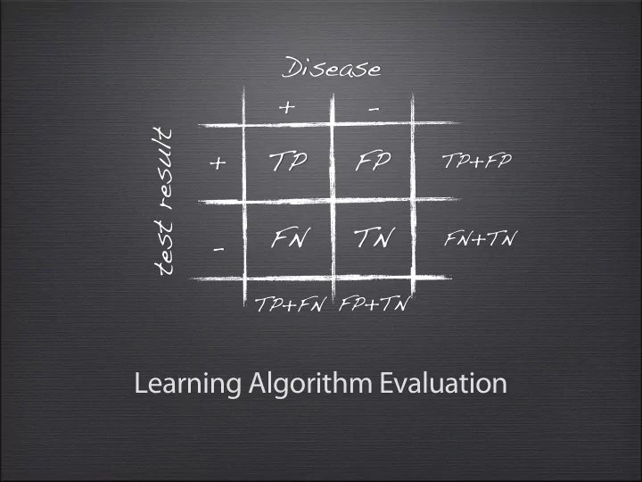
FN FP TN Disease t e s t r e s u l t

TP+FP FN+TN TP+FN FP+TN

Outline

Why?

• Overfitting

How?

• Holdout vs Cross-validation

What?

• Evaluation measures

Who wins?

• Statistical significance

Quiz

Is this a good model?

Overfitting

While it fits the training data perfectly, it may perform badly on unseen data. A simpler model may be better.

Outline

Why?

• Overfitting

How?

• Holdout vs Cross-validation

What?

• Evaluation measures

Who wins?

• Statistical significance

A first evaluation measure

• Predictive accuracy
• Success: instance’s class is predicted correctly
• Error: instance’s class is predicted incorrectly
• Error rate: #errors/#instances
• Predictive Accuracy: #successes/#instances
• Quiz
• 50 examples, 10 classified incorrectly
• Accuracy? Error rate?

Rule #1

Rule #1

Never evaluate on training data!

Holdout (Train and Test)

Holdout (Train and Test)

Holdout (Train and Test)

a.k.a. holdout set

Holdout (Train and Test)

a.k.a. holdout set

Holdout (Train and Test)

a.k.a. holdout set

Can I retry with other parameter settings?

Quiz

Rule #2

Rule #2

Never train/optimize on test data!

(that includes parameter selection)

You need a separate optimization set to tune parameters

Holdout (Train and Test)

OPTIMIZATION TESTING

Test data leakage

• Never use test data to create the classifier
• Can be tricky: e.g. social network
• Proper procedure uses three sets
• training set: train models
• ptimization/validation set: optimize algorithm

parameters

• test set: evaluate final model

Build final model on ALL data (more data, better model)

Holdout (Train and Test)

Making the most of data

• Once evaluation is complete, and algorithm/

parameters are selected, all the data can be used to build the final classifier

• Trade-off: performance <-> evaluation accuracy
• More training data, better model (but returns diminish)
• More test data, more accurate error estimate

Issues

• Small data sets
• Random test set can be quite different from training set

(different data distribution)

• Unbalanced class distributions
• One class can be overrepresented in test set
• Serious problem for some domains:
• medical diagnosis: 90% healthy, 10% disease
• eCommerce: 99% don’t buy, 1% buy
• Security: >99.99% of Americans are not terrorists

Balancing unbalanced data

Sample equal amounts from minority and majority class + ensure approximately equal proportions in train/test set

Stratified Sampling

Advanced class balancing: sample so that each class represented with approx. equal proportions in both subsets E.g. take a stratified sample of 50 instances:

Repeated holdout method

• Evaluation still biased by random test sample
• Solution: repeat and average results
• Random, stratified sampling, N times
• Final performance = average of all performances

Repeated holdout method

• Evaluation still biased by random test sample
• Solution: repeat and average results
• Random, stratified sampling, N times
• Final performance = average of all performances

Repeated holdout method

• Evaluation still biased by random test sample
• Solution: repeat and average results
• Random, stratified sampling, N times
• Final performance = average of all performances

TRAIN TEST TRAIN TEST TRAIN TEST

Repeated holdout method

• Evaluation still biased by random test sample
• Solution: repeat and average results
• Random, stratified sampling, N times
• Final performance = average of all performances

TRAIN TEST TRAIN TEST TRAIN TEST

0.86 0.74 0.8

Repeated holdout method

• Evaluation still biased by random test sample
• Solution: repeat and average results
• Random, stratified sampling, N times
• Final performance = average of all performances

TRAIN TEST TRAIN TEST TRAIN TEST

0.86 0.74 0.8 0.8

k-fold Cross-validation

Split data (stratified) in k-folds Use (k-1) for training, 1 for testing, repeat k times, average results

Cross-validation

• Standard method:
• stratified 10-fold cross-validation
• Experimentally determined. Removes most of

sampling bias

• Even better: repeated stratified cross-validation
• Popular: 10 x 10-fold CV, 2 x 3-fold CV

Leave-One-Out Cross-validation

• A particular form of cross-validation:
• #folds = #instances
• n instances, build classifier n times
• Makes best use of the data, no sampling bias
• Computationally very expensive

Outline

Why?

• Overfitting

How?

• Holdout vs Cross-validation

What?

• Evaluation measures

Who wins?

• Statistical significance

Some other Evaluation Measures

• ROC: Receiver-Operator Characteristic
• Precision and Recall
• Cost-sensitive learning
• Evaluation for numeric predictions
• MDL principle and Occam’s razor

ROC curves

• ROC curves
• Receiver Operating Characteristic
• From signal processing: tradeoff between hit rate and false

alarm rate over noisy channel

• Method:
• Plot True Positive rate against False Positive rate

Confusion Matrix

TPrate (sensitivity): FPrate (fall-out): +

• +
• TP

FN FP TN actual p r e d i c t e d

TP+FN FP+TN

true positive false positive false negative true negative

ROC curves

• ROC curves
• Receiver Operating Characteristic
• From signal processing: tradeoff between hit rate and false

alarm rate over noisy channel

• Method:
• Plot True Positive rate against False Positive rate
• Collect many points by varying prediction threshold
• For probabilistic algorithms (probabilistic predictions)
• Non-probabilistic algorithms have single point
• Or, make cost sensitive and vary costs (see below)

ROC curves

inst P(+) actual

1 0.8 + 2 0.5

• 3

0.45 + 4 0.3

• Predictions

TP FP

actually positive actually negative

FP

ROC curves

0.3 0.45 0.5 0.8

+ + + +

• +

+ +

• +

+

• +
• Thresholds

inst P(+) actual

1 0.8 + 2 0.5

• 3

0.45 + 4 0.3

• 0.3

0.45 0.5 0.8

TPrate

1 1 1/2 1/2

FPrate

1 1/2 1/2

Predictions TP FP

actually positive actually negative

FP

ROC curves

0.3 0.45 0.5 0.8

+ + + +

• +

+ +

• +

+

• +
• Thresholds

inst P(+) actual

1 0.8 + 2 0.5

• 3

0.45 + 4 0.3

• 0.3

0.45 0.5 0.8

TPrate

1 1 1/2 1/2

FPrate

1 1/2 1/2

Predictions TP FP

actually positive actually negative

FP

ROC curves

0.3 0.45 0.5 0.8

+ + + +

• +

+ +

• +

+

• +
• Thresholds

inst P(+) actual

1 0.8 + 2 0.5

• 3

0.45 + 4 0.3

• 0.3

0.45 0.5 0.8

TPrate

1 1 1/2 1/2

FPrate

1 1/2 1/2

Predictions TP FP

actually positive actually negative

FP

ROC curves

0.3 0.45 0.5 0.8

+ + + +

• +

+ +

• +

+

• +
• Thresholds

inst P(+) actual

1 0.8 + 2 0.5

• 3

0.45 + 4 0.3

• 0.3

0.45 0.5 0.8

TPrate

1 1 1/2 1/2

FPrate

1 1/2 1/2

Predictions TP FP

actually positive actually negative

FP

ROC curves

0.3 0.45 0.5 0.8

+ + + +

• +

+ +

• +

+

• +
• Thresholds

inst P(+) actual

1 0.8 + 2 0.5

• 3

0.45 + 4 0.3

• 0.3

0.45 0.5 0.8

TPrate

1 1 1/2 1/2

FPrate

1 1/2 1/2

Predictions TP FP

actually positive actually negative

FP

ROC curves

0.3 0.45 0.5 0.8

+ + + +

• +

+ +

• +

+

• +
• Thresholds

inst P(+) actual

1 0.8 + 2 0.5

• 3

0.45 + 4 0.3

• 0.3

0.45 0.5 0.8

TPrate

1 1 1/2 1/2

FPrate

1 1/2 1/2

Predictions TP FP

actually positive actually negative

FP

ROC curves

0.3 0.45 0.5 0.8

+ + + +

• +

+ +

• +

+

• +
• Thresholds

inst P(+) actual

1 0.8 + 2 0.5

• 3

0.45 + 4 0.3

• 0.3

0.45 0.5 0.8

TPrate

1 1 1/2 1/2

FPrate

1 1/2 1/2

Predictions TP FP

actually positive actually negative

FP

ROC curves

0.3 0.45 0.5 0.8

+ + + +

• +

+ +

• +

+

• +
• Thresholds

inst P(+) actual

1 0.8 + 2 0.5

• 3

0.45 + 4 0.3

• 0.3

0.45 0.5 0.8

TPrate

1 1 1/2 1/2

FPrate

1 1/2 1/2

Predictions TP FP

actually positive actually negative

FP

ROC curves

0.3 0.45 0.5 0.8

+ + + +

• +

+ +

• +

+

• +
• Thresholds

inst P(+) actual

1 0.8 + 2 0.5

• 3

0.45 + 4 0.3

• 0.3

0.45 0.5 0.8

TPrate

1 1 1/2 1/2

FPrate

1 1/2 1/2

Predictions TP FP

actually positive actually negative

FP

ROC curves

0.3 0.45 0.5 0.8

+ + + +

• +

+ +

• +

+

• +
• Thresholds

inst P(+) actual

1 0.8 + 2 0.5

• 3

0.45 + 4 0.3

• 0.3

0.45 0.5 0.8

TPrate

1 1 1/2 1/2

FPrate

1 1/2 1/2

Predictions TP FP

actually positive actually negative

FP

ROC curves

0.3 0.45 0.5 0.8

+ + + +

• +

+ +

• +

+

• +
• Thresholds

inst P(+) actual

1 0.8 + 2 0.5

• 3

0.45 + 4 0.3

• 0.3

0.45 0.5 0.8

TPrate

1 1 1/2 1/2

FPrate

1 1/2 1/2

Predictions TP FP

actually positive actually negative

FP

ROC curves

0.3 0.45 0.5 0.8

+ + + +

• +

+ +

• +

+

• +
• Thresholds

inst P(+) actual

1 0.8 + 2 0.5

• 3

0.45 + 4 0.3

• 0.3

0.45 0.5 0.8

TPrate

1 1 1/2 1/2

FPrate

1 1/2 1/2

Predictions TP FP

actually positive actually negative

FP

inst P(+) actual

1 0.8 + 2 0.5

• 3

0.45 + 4 0.3

• Predictions

TP FP

• Rank probabilities, start curve in (0,0)
• Start curve in (0,0), move down probability list
• If next n are actually +: move up n, else move n right

ROC curves Alternative method

inst P(+) actual

1 0.8 + 2 0.5

• 3

0.45 + 4 0.3

• Predictions

TP FP

• Rank probabilities, start curve in (0,0)
• Start curve in (0,0), move down probability list
• If next n are actually +: move up n, else move n right

ROC curves Alternative method

inst P(+) actual

1 0.8 + 2 0.5

• 3

0.45 + 4 0.3

• Predictions

TP FP

• Rank probabilities, start curve in (0,0)
• Start curve in (0,0), move down probability list
• If next n are actually +: move up n, else move n right

ROC curves Alternative method

inst P(+) actual

1 0.8 + 2 0.5

• 3

0.45 + 4 0.3

• Predictions

TP FP

• Rank probabilities, start curve in (0,0)
• Start curve in (0,0), move down probability list
• If next n are actually +: move up n, else move n right

ROC curves Alternative method

inst P(+) actual

1 0.8 + 2 0.5

• 3

0.45 + 4 0.3

• Predictions

TP FP

• Rank probabilities, start curve in (0,0)
• Start curve in (0,0), move down probability list
• If next n are actually +: move up n, else move n right

ROC curves Alternative method

inst P(+) actual

1 0.8 + 2 0.5

• 3

0.45 + 4 0.3

• Predictions

TP FP

• Rank probabilities, start curve in (0,0)
• Start curve in (0,0), move down probability list
• If next n are actually +: move up n, else move n right

ROC curves Alternative method

inst P(+) actual

1 0.8 + 2 0.5

• 3

0.45 + 4 0.3

• Predictions

TP FP

• Rank probabilities, start curve in (0,0)
• Start curve in (0,0), move down probability list
• If next n are actually +: move up n, else move n right

ROC curves Alternative method

ROC curves Real Example

• Jagged curve—one set of test data
• Smooth curve—use cross-validation

Cross-validation and ROC curves

• Simple method of getting a ROC curve using cross-

validation:

• Collect probabilities for instances in test folds
• Sort instances according to probabilities
• a ROC curve for each fold, average afterwards
• This method is implemented in WEKA
• For n-class problems:
• make 1 class positive, others negative
• build ROC curve, repeat n times
• take weighted average (by class weight)

ROC curves Method selection

• Overall: use method with largest Area

Under ROC curve (AUROC)

• If you aim to cover just 40% of true

positives in a sample: use method A

• Large sample: use method B
• In between: choose between A and B with

appropriate probabilities

Precision and Recall

• Precision: TP/(TP+FP)
• Recall: TP/(TP+FN)

(= TPrate)

+

• +
• TP

FN FP TN actual p r e d i c t e d

TP+FP TP+FN

true positive false positive false negative true negative

E.g. Google‘s 1st result page: Precision: % returned pages that are relevant Recall: % relevant pages that are returned

Precision and Recall

• Precision and recall constitute a trade-off
• Often aggregated:
• 3-point average: avg. precision at 20, 50, 80% recall
• F-measure: harmonic average of precision and recall:

(2×recall×precision)/(recall+precision)

• Area under precision-recall curve

Cost Sensitive Learning

Different Costs

• In practice, TP and FN errors incur different costs
• Examples:
• Medical diagnostic tests: does X have leukemia?
• Loan decisions: approve mortgage for X?
• Promotional mailing: will X buy the product?
• …
• Add cost matrix to evaluation that weighs TP,FP,...

pred + pred - actual +

cTP = 0 cFN = 100

actual -

cFP = 1 cTN = 0

Cost-sensitive classification

• Probabilistic algorithms: calculate costs afterwards
• Instead of predicting most likely class, predict the one that

has the smallest expected misclassification cost

• e.g. p+ = 0.8, p-= 0.2
• cost+: [p+,p-]x[cTP,cFP] = 1
• cost- : [p+,p-]x[cFN,cTN] = 0.8
• Non-probabilistic algorithms: introduce costs during

training:

• Re-sample instances according to costs: higher % of negatives: FP<FN
• Weight instances according to costs

pred + pred - actual +

cTP = 0 cFN = 1

actual -

cFP = 5 cTN = 0

Evaluating numeric prediction

• Numeric predictions:
• Actual target values: a1 a2 …an
• Predicted target values: p1 p2 … pn
• Mean-squared error:
• Root mean-squared error:
• Mean absolute error:
• Less sensitive to outliers
• Sometimes relative error values more appropriate
• e.g. 10% for an error of 50 when predicting 500

Correlation coefficient

• Measures the statistical correlation between the predicted

values and the actual values

• Scale independent, between –1 (inverse correlation) and

+1 (perfect correlation)

• Error: smaller is better, correlation: larger is better

Which measure?

A B C D Root mean-squared error 67.8 91.7 63.3 57.4 Mean absolute error 41.3 38.5 33.4 29.2 Root rel squared error 42.2% 57.2% 39.4% 35.8% Relative absolute error 43.1% 40.1% 34.8% 30.4% Correlation coefficient 0.88 0.88 0.89 0.91

D best C second-best A, B arguable

• Classification: depends on application
• e.g. information retrieval: precision/recall very important
• Results may vary, especially for multi-class problems
• Regression: best look at all of them
• Many outliers in data: avoid squared error measures
• Otherwise, relative scores don’t differ much:

The MDL principle

• MDL stands for minimum description length
• The description length is defined as:

L(H) : space required to describe a hypothesis + L(D|H) : space required by using the hypothesis

• Examples
• L(H): model, L(D|H): encoded data
• Classifier: L(H): classifier, L(D|H): mistakes on the training data
• Aim: we seek a classifier with minimal DL
• MDL principle is a model selection criterion

Model selection criteria

• Model selection criteria attempt to find a good

compromise between:

• The complexity of a model
• Its prediction accuracy on the training data
• Reasoning: a good model is a simple model that

achieves high accuracy on the given data

• Also known as Occam’s Razor :

the best theory is the smallest one that describes all the facts

William of Ockham, born in the village of Ockham in Surrey (England) around 1285, was the most influential philosopher of the 14th century and a controversial theologian.

Elegance vs. errors

• Theory 1: very simple, elegant theory that explains the

data almost perfectly

• Theory 2: significantly more complex theory that

reproduces the data without mistakes

• Theory 1 is probably preferable
• Classic example: Kepler’s three laws on planetary motion
• Less accurate than Copernicus’s latest refinement of the

Ptolemaic theory of epicycles

MDL and compression

• MDL principle relates to data compression:
• The best theory is the one that compresses the data the most
• I.e. to compress a dataset we generate a model and then store

the model and its mistakes

Discussion of MDL principle

• Advantage: makes full use of the training data when

selecting a model

• Disadvantage 1: appropriate coding scheme/prior

probabilities for theories are crucial

• Disadvantage 2: no guarantee that the MDL theory is the
• ne which minimizes the expected error
• Note: Occam’s Razor is an axiom!
• Epicurus’ principle of multiple explanations: keep all theories

that are consistent with the data

Outline

Why?

• Overfitting

How?

• Holdout vs Cross-validation

What?

• Evaluation measures

Who wins?

• Statistical significance

Comparing data mining schemes

• Which of two learning algorithms performs better?
• Note: this is domain/measure dependent!
• Obvious way: compare 10-fold CV estimates
• Problem: variance in estimate
• Different random sample, different estimate
• Variance can be reduced using repeated CV
• However, we still don’t know whether results are reliable

Significance tests

• Significance tests tell us how confident we can be that there

really is a difference

• Null hypothesis: there is no “real” difference (meanA=meanB)
• Alternative hypothesis: there is a difference
• A significance test measures how much evidence there is in favor
• f rejecting the null hypothesis
• E.g. 10 cross-validation scores: B better than A???

Algoritme A Algoritme B perf P(perf) mean A mean B

x x x xxxxx x x x x x xxxx x x x

Paired t-test

• No normal distribution: we need more than the means
• Student’s t-test tells whether the means of two samples (e.g.,

k cross-validation scores) are significantly different

• Use a paired t-test when individual samples are paired
• i.e., they use the same randomization
• Same CV folds are used for both algorithms

Algoritme A Algoritme B perf P(perf) mean A mean B

x x x xxxxx x x x x x xxxx x x x

Not a normal distribution (although it will be for large k,>100)

• > Student’s distribution with

k-1 degrees of freedom

Paired T-test

• Fix a significance level α
• Significant difference at α% level implies (100-α)% chance that there really

is a difference. For scientific work: 0,5% or smaller (>99,5% certainty)

• Divide α by two (two-tailed test)
• We do not know whether meanA>meanB or vice versa
• Look up the z-value corresponding to α/2:
• If t ≤ –z or t ≥ z: difference is significant
• null hypothesis can be rejected

α

z 0,1% 4.3 0,5% 3.25 1% 2.82 5% 1.83 10% 1.38 20% 0.88

Table of confidence intervals for Student’s distribution with 9 (10-1) degrees of freedom

• diff. of means
• diff. of variances

α

z 0,1% 4.3 0,5% 3.25 1% 2.82 5% 1.83 10% 1.38 20% 0.88

Paired T-test

Unpaired observations

• If CV estimates are from different randomizations

(different folds), they are no longer paired

• In general: comparing k-fold and j-fold CV results
• Use un-paired t-test with min(k , j) – 1 degrees of freedom
• The t-statistic becomes:

Summary

• Use holdout method for LARGE data
• Use Cross-validation for small data, with stratified

sampling

• Don’t use test data for parameter tuning - use

separate optimization/validation data

• Use appropriate evaluation measures
• Consider costs when appropriate
• Perform a statistical significance test to choose

between algorithm