LIC-Based Regularization of Multi-Valued Images David Tschumperl - - PowerPoint PPT Presentation

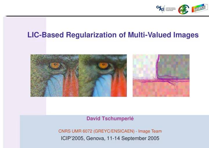
LIC-Based Regularization of Multi-Valued Images

David Tschumperlé

CNRS UMR 6072 (GREYC/ENSICAEN) - Image Team

ICIP’2005, Genova, 11-14 September 2005

Data Regularization

• Aim of regularization consists in transforming a noisy signal into a more regular
• ne, while preserving the important image informations (discontinuities).

Regularization of a noisy 1D signal Regularization of a noisy 2D image

• Several regularization methods exist in the litterature.

⇒ Non-linear diffusion PDE’s are particularly efficient for this task.

PDE Framework in Image Processing

• PDE = Partial Differential Equation :

∂I ∂t = ∂2I ∂x2 + ∂2I ∂y2

• Using PDE’s in Image Processing :
• I represents the data (1D signals or 2D/3D images) we want to process.
• t is an extra time variable corresponding to the PDE iterations.

⇒ Iterative Algorithm

• One starts from an image I(t=0) which evolves until convergence, or after a

finite number of iterations (t = tend).        I(t=0) = I0

∂I(x,y,t) ∂t

= β(x,y,t)

PDE’s and Image Regularization

• Convolution and linear PDE’s (Koenderink[84], Alvarez-Guichard-etal[92], ...) :

I(t) = I(t=0) ∗ Gσ where Gσ = 1 4πt e−x2+y2

4t

⇐ ⇒ ∂I ∂t = ∆I

• Nonlinear PDE’s (Perona-Malik[90], Alvarez [92], ...) :

∂I ∂t = div (c(∇I) ∇I) with c : R − → R

Noisy scalar image linear PDE Perona-Malik PDE

PDE Regularization of Scalar Images

• A wide range of PDE-based methods have been proposed since Perona-Malik[90],

for scalar image regularization I : Ω → R.

(Alvarez, Aubert, Barlaud, Blanc-Feraud, Charbonnier, Chan, Cohen, Deriche, Kornprobst, Malladi, Munford, Morel, Nordström, Osher, Perona-Malik, Rudin, Sapiro, Sochen, Weickert,...) Noisy scalar image I : Ω → R Regularized image, using PDE

PDE Regularization of Multivalued Images

• Image I : Ω → N of multivalued points : vectors (N = Rn), matrices (N =

Mn). (Blomgren-Chan[98], Kimmel-Malladi-Sochen[98], Sapiro-Ringach[96], Tschumperle-

Deriche[01,03], Weickert[97,03], ...) Color Image (N = R3) Scalar PDE, channel by channel Multivalued PDE Noisy 2D vector field (N = R2) Regularized field

Principle of PDE-based Regularization

• PDE regularization is mainly based on local image smoothing.
• Local image smoothing is done as follows :

– On a edge, smoothing is done only along the edge, to preserve it. – On homogeneous regions, smoothing is done isotropically (in all directions).

How the smoothing is done ?

• Let I : Ω → Rn be a noisy multi-valued image.
• Smoothing depends on the local geometry of I. Computation of the smoothed

structure tensor field Gσ = G ∗ Gσ : ∀(x, y) ∈ Ω, G(x,y) =

i ∇Ii∇IT i

• Eigenvalues λ+, λ− and eigenvectors θ+, θ− of G describe the local configuration
• f I at point (x, y).

⇒ Definition of a diffusion tensor field T from G that will tell how the smoothing is

• performed. For instance :

T = f1(λ+ + λ−) θ−θT

− + f2(λ+ + λ−) θ+θT +

with      f1(s) =

1 1+sp

f2(s) =

1 √1+sq

How the smoothing is done ? (2)

• Then, the smoothing itself is performed by the application of one or several PDE

iterations : ∂Ii ∂t = div (T∇Ii)

• r

∂Ii ∂t = trace (THi) ⇒ The smoothing behavior of the PDE process follows then the tensor field T :

Application of a diffusion PDE on a color image, following a synthetic tensor field T.

⇒ Efficient regularization of images when T is correctly defined.

LIC : Line Integral Convolution

• LIC has been proposed by Cabral & Leedom in 93 as a method to visualize vector

flows F : R2 → R2. ⇒ Starting from a pure noisy image Inoise, compute for each pixel X = (x, y) an averaging of the image intensities along integral curves CX of F : ∀(x, y) ∈ Ω, ILIC

(x,y) = 1

N +∞

−∞

f(p) Inoise(CX

(p)) dp

where        CX

(0)

= X

∂CX

(a)

∂a

= F(CX

(a))

• From smoothing purposes, on may choose f(p) to be gaussian.

LIC : Line Integral Convolution (2)

• Smooth locally the image in different directions, following a vector field.

⇒ This suggests this can be used for PDE-based smoothing following a tensor field.

Contribution : Mixing LIC’s and PDE’s

• We propose a LIC-based process that smoothes an image along a tensor field T,

where T is defined as in the PDE-based regularization processes.

• We decompose a smoothing along a tensor T into several smoothing processes

along vectors wθ = TUθ, where Uθ = (cos θ, sin θ) : – If T(X) is isotropic then wθ

(X) = αUθ.

– If T(X) is anisotropic and directed along Uθ, then wθ

(X) ≃ αUθ.

– If T(X) is anisotropic and orthogonal to Uθ, then wθ

(X) ≃ ˜

0. ⇒ The more Uθ represents a part of T, the higher will be the norm wθ.

LIC-based smoothing along diffusion tensors

• One replace one PDE iteration by a multiple LIC computation :

Iregul

(X)

= 1 N π dtwθ

(X)

−dtwθ

(X)

f(a) Inoisy(Cθ

(X,a)) da dθ

where f() is a gaussian, N = f(a)dadθ, and dt is the overall smoothing strength.

• Cθ

(X,0)

= X

∂Cθ ∂a (X, a)

= wθ(Cθ

(X,a)) = T(Cθ (X,a)) U(θ)

Properties ⇒ Maximum principle is verified (only averaging of pixel values). ⇒ Very stable and fast algorithm compared to classical PDE implementations : Time step (dt) can be large, process remains stable. ⇒ Corners and curved structures are particularly well preserved.

(a) Original image (b) PDE-based (explicit Euler scheme) (c) LIC-based

Preservation of curved structures

• Smoothing processes are done around the corners, taking into account the

curvature of the image structures.

• LIC’s naturally provide sub-pixel accuracy for the smoothing.

Applications : Image Denoising

“Baboon” (detail) 512x512 (1 iter., 19s) “Tunisia” (detail) 555x367 (1 iter., 11s)

Applications : Image Denoising (2)

“Lena” (detail) 256x256 (1 iter., 6.4s) “Chris” (detail) 293x306 (1 iter., 5.6s)

Applications : Image Denoising (3)

“Penguin” (detail) 355x287 (1 iter., 12.8s) “Farm” (detail) 460x365 (1 iter., 26s)

Applications : Image Inpainting and Reconstruction

“Parrot” 500x500 (200 iter., 4m11s) “Owl” 320x246 (10 iter., 1m01s)

Applications : Image Interpolation

(a) Original color image (b) Bloc interpolation (b) Linear interpolation (b) Bicubic interpolation (b) PDE-based interpolation

Applications : Image Interpolation (2)

“Nude” (1 iter., 20s) “Forest” (1 iter., 5s)

Conclusions & Perspectives

• Very simple and efficient regularization process for multi-valued images.
• Mix between PDE and LIC based techniques.

⇒ Perspectives : ’Curvature-preserving PDE’ corresponding to our tensor-directed LIC formulation :

Fast Anisotropic Smoothing of Multi-Valued Images using Curvature-Preserving PDE’s.

• D. Tschumperlé

Research Report : “Les cahiers du GREYC”, No 05-01, January 2005.