Modeling And Visualizing Fire Without Getting Burned MCSD Seminar - - PowerPoint PPT Presentation

modeling and visualizing fire without getting burned
SMART_READER_LITE
LIVE PREVIEW

Modeling And Visualizing Fire Without Getting Burned MCSD Seminar - - PowerPoint PPT Presentation

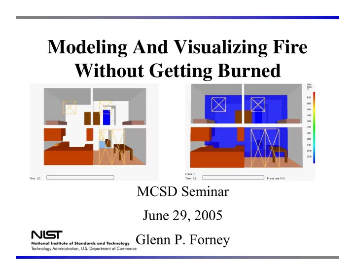
Modeling And Visualizing Fire Without Getting Burned MCSD Seminar June 29, 2005 Glenn P. Forney Overview Fire Models Fire modeling applications Gaining insight through visualization Smokeview Visualization Team FDS


slide-1
SLIDE 1

Modeling And Visualizing Fire Without Getting Burned

MCSD Seminar June 29, 2005 Glenn P. Forney

slide-2
SLIDE 2

Overview

  • Fire Models
  • Fire modeling applications
  • Gaining insight through visualization
slide-3
SLIDE 3

Smokeview Visualization “Team”

Glenn Forney Kevin McGrattan Howard Baum Ron Rehm Anthony Hamins – experimental validation Steve Kerber – forced ventilation Greg Linteris – fundamental fire Physics Ruddy Mell Ron Rehm Urban-wildland interface problem Dan Madrzykowski Bob Vettori Doug Walton Fire reconstructions

and others… FDS computational model

Kuldeep Prasad – multi-mesh Chuck Bouldin - parallelization

Smokeview visualization

slide-4
SLIDE 4

The Purpose of Computing is Insight Not Numbers - R. W. Hamming

Influence on visualization and Smokeview

slide-5
SLIDE 5

Fire Models

  • Can provide insight into complex phenomena

within a fire scenario including Flame spread Gas Conc. Fuel package Smoke HRR Ventilation Suppression Radiation

  • Can provide a tool for understanding

Fire behavior under various ventilation conditions

slide-6
SLIDE 6

Single Equation Models

Hand (or simple computer) calculations

– Heat release rate – Flame height – Minimum Flashover HRR – T-squared Fire Growth

  • Predicting Time to Flashover
slide-7
SLIDE 7

Flame Height

D Q Lf 02 . 1

  • 23

. =

5 / 2

&

Trash can HRR = 50 kW Trash can diameter = 0.3 m (1 ft) Estimated Trash Can Flame Height = 0.8 m (2.5 ft) P 138 JQ

slide-8
SLIDE 8

Zone Models

(ODE models)

  • Divide room into two zones

Hot Upper Zone Cool Lower Zone

slide-9
SLIDE 9

Zone models

  • Two primary control volumes

– Upper / lower layers

  • Conditions assumed uniform in each layer
  • Correlations

– Combustion – Plume flow – Vent flow (entrainment)

Hot Upper Zone Cool Lower Zone

slide-10
SLIDE 10

Zone models

radiation entrainment

ylay

f

m &

f

q &

v

q &

v

m &

convection c

q &

r

q &

v

q &

v

m &

slide-11
SLIDE 11

Zone Modeling Equations

U U L L

T T R P ρ ρ = =

U U V U

T m c E =

L L

m dt dm & =

L L L

q dt dV P dt dE & = +

U U

m dt dm & =

U U U

q dt dV P dt dE & = +

Internal energy work enthalpy

State Equations

Ideal Gas Law Internal Energy

L L V L

T m c E = Conservation of mass and energy

slide-12
SLIDE 12

Zone models

Governing Equations:

) + ( V 1

  • γ

=

U L q

q dt dP & &

Pressure:

)

  • (

γ A 1

  • =

room

dt dP V q P dt dy

U U abs lay

&

Layer interface:

) V

  • )

T m c

  • ((

1 =

X X X p

dt dP q m c dt dT

X X p X

& &

Upper/Lower Layer Temperature:

slide-13
SLIDE 13

Zone Modeling Equations

⎟ ⎟ ⎟ ⎟ ⎟ ⎠ ⎞ ⎜ ⎜ ⎜ ⎜ ⎜ ⎝ ⎛ =

U L U

T T V P x

) (x f dt dx =

“Small” changes in P, VU, TL, TU Large changes in dP/dt Stiff ODE solvers required for solution (use DASSL)

slide-14
SLIDE 14

Zone model visualization

slide-15
SLIDE 15

Zone to Field Models

slide-16
SLIDE 16

Field models

slide-17
SLIDE 17

Fire Dynamics Simulator and Smokeview

Version 1 release, February 2000 Version 4 release, November 2004 http://fire.nist.gov/fds

slide-18
SLIDE 18

Fire Modeling Applications

slide-19
SLIDE 19

Fuel Spray (Walton, Floyd)

slide-20
SLIDE 20

Rack Storage Fire

slide-21
SLIDE 21

WTC Phase 1, Test 5, West Aspirated TCs Time (s)

1000 2000 3000

Temperature (C)

200 400 600 800 1000

365 cm (Exp) 215 cm (Exp) 34 cm (Exp) 365 cm (FDS) 215 cm (FDS) 34 cm (FDS)

FDS Validation Experiment 3 MW Fire, 23’x12’x12’ Compartment, 1 hour burn

slide-22
SLIDE 22
slide-23
SLIDE 23

Visualizing Fire Data

Fire Dynammics Simulator (FDS) - Modeling Fire Data

slide-24
SLIDE 24

Software Used With Smokeview

  • OpenGL – 3D low level graphics API
  • GLUT – graphics library utility toolkit
  • GLUI – user interface toolkit implementing

dialog boxes using GLUT and OpenGL

  • C
  • Fortran 90
slide-25
SLIDE 25

Software Used With Smokeview (Cont)

  • GD – image library
  • Pnglib – image library
  • Zlib – compression library
  • Jpeglib – image library
slide-26
SLIDE 26

Who is Using FDS and Smokeview?

1) Developers

Diagnose problems with Physics and Numerics of FDS

slide-27
SLIDE 27

Who is Using FDS and Smokeview?

Study effects of fire dynamics Cherry Road LODD Incident December 1999 Litigation, Forensic studies, Fire Protection Engineers, Architects, Regulatory agencies NRC, DOE, …

2) Engineers/Scientists

slide-28
SLIDE 28

Who is Using FDS and Smokeview?

3) Fire Fighters (trainees)

Fight fire “on the computer”

slide-29
SLIDE 29

Visualization Overview

  • load data
  • specify geometry
  • Light scene
  • move, translate

and scale geometry

x M M

n 1L

Mi – rotation, translation or scaling matrix transformations x – position vector Motion Color Structure

slide-30
SLIDE 30

Drawing

  • Specify vertices
  • Draw objects (connect vertices)
  • Move objects
  • Project objects onto 2D plane
  • Transfer 2D plane onto a portion of the

computer screen

slide-31
SLIDE 31

Drawing Shapes

slide-32
SLIDE 32

Lighting

slide-33
SLIDE 33

Smokeview Shading Example

Shaded Unshaded

slide-34
SLIDE 34

Smokeview Shading Example

Shaded isosurface Unshaded slice

slide-35
SLIDE 35

Lighting/Shading

Light source normals

Lighting

  • Adds more realism to 3D scenes
  • Computed using normal vectors

light source direction vectors Observer

slide-36
SLIDE 36

Specifying Normals

(Perpendiculars)

One normal per triangle glNormal3f(nx,ny,nz); glVertex3f(ux,uy,uz); glVertex3f(vx,vy,vz); glVertex3f(wx,wy,wz); (facet shape) n = (u-v) x (w-v) u v w n

slide-37
SLIDE 37

Specifying Normals (Cont)

(Perpendiculars)

One normal per vertex glNormal3f(nx1,ny1,nz1); glVertex3f(x1,y1,z1); glNormal3f(nx2,ny2,nz2); glVertex3f(x2,y2,z2); glNormal3f(nx3,ny3,nz3); glVertex3f(x3,y3,z3); (smooth shape) u v w

slide-38
SLIDE 38

Drawing a Smokeview Scene

  • Particles
  • Shaded contours (slice files)
  • 3D contours (isosurface files)
  • 3D Smoke
slide-39
SLIDE 39

Particles

glPointSize(partpointsize); glBegin(GL_POINTS); for (n = 0; n < nsmokepoints; n++) { glColor4fv(rgb[itpoint[n]]); glVertex3f(xplts[xpoints[n]], yplts[ypoints[n]],zplts[zpoints[n]]); } glEnd();

slide-40
SLIDE 40

Slices - 2D Contours

slide-41
SLIDE 41

2D Contours (Cont)

10 5 5 5 5 10

slide-42
SLIDE 42

2D Contours (Cont)

10 5 5 5 5 10

Triangulate so that all hypotenuses follow level curves

slide-43
SLIDE 43

Slices 2D Contours - Example

slide-44
SLIDE 44

Computing 3D Contours (isosurfaces)

Marching Cube Algorithm

  • Divide domain into a number of cubes
  • For each cube determine where isosurface crosses cube
  • At each corner of cube data is either above or below

isosurface level – 256 cases

  • Above isosurface level

3 of 15 cases

slide-45
SLIDE 45

3D Contours - Example

Outline Solid

slide-46
SLIDE 46

3D Contours - Example

Multiple normals for each vertex Single normal for each vertex

slide-47
SLIDE 47

Transparency - Example

Transparent Solid

slide-48
SLIDE 48

Visualizing Smoke

tracer particles 3d contours realistic/3D smoke

slide-49
SLIDE 49

Simple Smoke Visualization Strategy

Observer

Assume “ambient” light source behind smoke

Mix smoke color with background scene color Background scene

slide-50
SLIDE 50

Advanced Smoke Visualization Strategy

Observer

“Ambient” light source behind smoke

Mix smoke color with background scene color Background scene Directional light source

slide-51
SLIDE 51

Examples

Sun behind clouds Sun above clouds Diffuse/Ambient Light

slide-52
SLIDE 52

3D Smoke

Using Transparency to Visualize Smoke Physics-based computation of smoke transparency Front View Side View

slide-53
SLIDE 53

3D Smoke

Using Transparency to Visualize Smoke Physics-based computation of smoke transparency α − οbscuration Δx - distance between adjacent grid planes si- soot density αi = 1 - exp(-ksiΔx) - Beer’s law

slide-54
SLIDE 54

3D Smoke

  • Smokeview adjusts each αi

in real time for non-axis aligned view distances using: x x Δ Δ

− − =

/ ˆ

) 1 ( 1 ˆ α α

  • Smoke may be drawn faster by skipping planes

(need to adjust α’s for planes that remain)

2 / ˆ = Δ Δ X X

2 2

2 ) 1 ( 1 ˆ α α α α − = − − =

slide-55
SLIDE 55

Benchmark Exercise: Under-ventilated Compartment

slide-56
SLIDE 56

3D Smoke

Reality Check

slide-57
SLIDE 57

Future Work

Possible future directions for Smokeview

slide-58
SLIDE 58

Representing Data With Color

slide-59
SLIDE 59

Representing Data With Color

slide-60
SLIDE 60

Representing Data With Color

3D color “space”

slide-61
SLIDE 61

Representing Data With Color

“rainbow colorbar” 3D color “space”

slide-62
SLIDE 62

Simulating Thermal Imagers

Determine colorbar appropriate for use with a thermal imager How does a thermal imager respond to

  • temperature,
  • gas composition
slide-63
SLIDE 63

Exploiting Texture Mapping and Tours

slide-64
SLIDE 64

Beyond the CPU

Programming the GPU

Use the video card (GPU) to perform scientific computations Why? Pseudo code for 3D smoke visualization

for(i=0;i<ni;i++){ for(j=0;j<nj;j++){ correct α at each grid node { }

CPU - serial GPU - parallel

slide-65
SLIDE 65

Summary

  • Not enough to run a fire model (or any model)
  • Visualization is a useful tool for analyzing data

and gaining insight into the phenomena being studid glenn.forney@nist.gov