
SLIDE 1
P e t e r S k a n d s ( C E R N T H )
N LO an d H e lic i ty Am p l i t u d es i n VIN C IA
W o r k s h o p o n P a r t o n S h o w e r s a n d R e s u m m a t i o n I P P P, D u r h a m , J u l y 2 0 1 3
0.6 0.7 0.8 0.9 0.95 1.05 1.1 1.2 1.2 1.3 1.3 1.4 1.4 1.5 1.5
- 8
- 6
- 4
- 2
- 8
- 6
- 4
- 2
lnHyijL lnHyjkL
QE=mD HstrongL
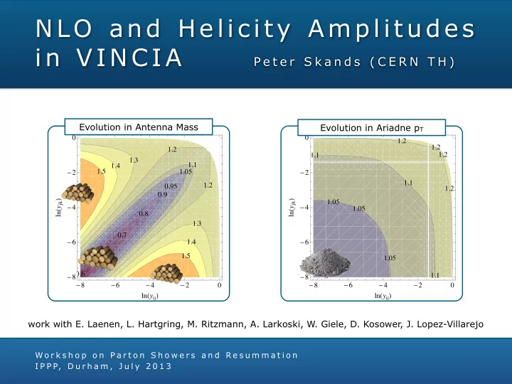
Evolution in Antenna Mass
1.05 1.1 1.1 1.1 1.2 1.2 1.2 1.2
- 8
- 6
- 4
- 2
- 8
- 6
- 4
- 2
lnHyijL lnHyjkL
QE=2pT HstrongL
1.05 1.05
Evolution in Ariadne pT work with E. Laenen, L. Hartgring, M. Ritzmann, A. Larkoski, W. Giele, D. Kosower, J. Lopez-Villarejo