Not Smooth High degree approximation Explicit y=f(x) Implicit - - PowerPoint PPT Presentation

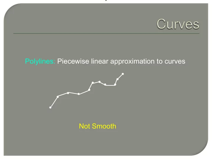
Polylines: Piecewise linear approximation to curves Not Smooth

High degree approximation

• Explicit

y=f(x)

• Implicit

f(x,y)=0

• Parametric

x=x(t), y=y(t)

Explicit Representation

• Essentially a function plot over some interval

x ∈ a,b

[ ]

y = f (x)

• Simple to compute and plot
• Simple to check whether point lies on curve
• Cannot represent closed and multi-value curves

Implicit Representation

• Define curves implicitly as solution of equation

system !Straight line in 2D: ax + by +c = 0

! Circle of radius R in 2D: x2 + y2 − R2 = 0 ! Conic Section: Ax2 + 2Bxy +Cy2 + 2Dx + 2Ey + F = 0

• Simple to check whether point lies on curve
• Can represent closed and multi-value curves

Parametric Curves

• Describe position on the curve by a parameter

u ∈ R

⇒ 2D Curve c(u) = {x(u), y(u)} e.g.,line :c(u) = (1−u)a +ub

a b 1 u

• Hard to check whether point lies on curve
• Simple to render
• Can represent closed and multi-value curves

Parametric Curves

Parametric curves form a rich variety of free form smooth curves They are modeled as piecewise polynomials and have two aspects:

• Interpolation
• Approximation

“Splines”

Parametric Curves

Splines

Parametric Curves

Cubic Splines

∑

= −

= ≤ ≤ + + + =

4 1 1 2 1 3 4 2 3 2 1

) (

i i it

B t t t t B t B t B B t P

∑ ∑

= − = −

= =

4 1 1 4 1 1

) ( ) (

i i iy i i ix

t B t y t B t x

∑

= −

+ + = − =

4 1 2 4 1 3 2 2

3 2 ) 1 ( ) ( '

i i i

t B t B B t i B t P

Parametric Curves

P1 t1 P1’ P2’ P2 t2

Let t1=0 P(0)=P1, P(t2)=P2 P'(0)=P1’, P’(t2)=P2’

Cubic Splines

Parametric Curves

P1 t1 P1’ P2’ P2 t2 Cubic Splines

' 3 2 ) 1 ( ) ( ' ' ) 1 ( ) ( ' ) ( ) (

2 2 2 4 1 2 3 2 4 1 2 2 1 2 4 1 2 2 3 2 4 2 2 3 1 2 2 1 4 1 1 2 1 1

2 2

P t B t B B t i B t P P B t i B P P t B t B t B B t B t P P B P

t t i i i t i i i t t i i i

= + + = − = = = − = = + + + = = = =

= = − = = − = = −

∑ ∑ ∑

Parametric Curves

Cubic Splines

2 2 ' 2 2 2 ' 1 3 2 2 1 4 2 ' 2 2 ' 1 2 2 1 2 3 ' 1 2 1 1 4 3 2 1

t P t P t ) P

• 2(P

B t P

• t

2P

• t

) P

• 3(P

B , P B , P B B and B B B for Solving + + = = = =

Here P1 and P2 give the position of the endpoints and P1’ and P2’ give the direction of the tangent vectors.

P1 t1 P1’ P2’ P2 t2

Parametric Curves

3 2 2 2 2 2 1 3 2 2 1 2 2 2 2 1 2 2 1 2 1 1

' ' ) ( 2 ' ' 2 ) ( 3 ' ) ( t t P t P t P P t t P t P t P P t P P t P ⎟ ⎟ ⎠ ⎞ ⎜ ⎜ ⎝ ⎛ + + − + ⎟ ⎟ ⎠ ⎞ ⎜ ⎜ ⎝ ⎛ − − − + + =

Thus, given the two end-points and the tangent vectors

• ne can compute the cubic spline.

Cubic Splines P1 t1 P1’ P2’ P2 t2

Parametric Curves

Joining of Segments 2 SEGMENTS: P1 P2 P3 (Points) P1’ P2’ P3’ (Tangents) P2’ is determined through the continuity condition

t1 t2 t3 Cubic Splines

Parametric Curves

Piecewise Spline of degree k has continuity

• f order (k-1) at the internal joints.

Thus Cubic Splines have second order continuity i.e. P2”(t) is continuous over the joint

t1 t2 t3 Cubic Splines

Parametric Curves

t1 t2 t3 Cubic Splines

( ) ( )

2 3 1 3 2 4 3 3 2 4 2 4 1 2 1 3

2 2 6 , 2 2 6 ) 2 )( 1 ( ) ( ' '

seg seg ' ' ' ' i i i

B B t B So B P segment Second B t B P segment First t t at t t t t B i i t P = + = + = = ≤ ≤ − − = ∑

= −

Substitute the expressions for B4 and B3

Parametric Curves

t1 t2 t3 Cubic Splines

( )

[ ]

( )

) ( ) ( 3 ' ' ' ) ( 2 ) ( ) ( 3 ' ' ) ( 2 '

1 2 2 3 2 3 2 2 3 2 3 2 1 2 2 3 3 1 2 2 3 2 3 2 2 3 2 3 2 2 2 3 1 3

P P t P P t t t P P P t t t t P P t P P t t t P t P t t P t − + − = ⎥ ⎥ ⎥ ⎦ ⎤ ⎢ ⎢ ⎢ ⎣ ⎡ + − + − = + + +

Parametric Curves

In general, for the kth and (k+1)th segment (1≤k≤n-2)

[ ]

( )

) ( ) ( 3 ' ' ' ) ( 2

1 2 2 1 2 2 1 2 1 2 1 1 2 1 2 k k k k k k k k k k k k k k k

P P t P P t t t P P P t t t t − + − = ⎥ ⎥ ⎥ ⎦ ⎤ ⎢ ⎢ ⎢ ⎣ ⎡ +

+ + + + + + + + + + + + +

Set of n-2 equations form a linear system for the tangent vectors Pk’

Cubic Splines

Parametric Curves

Cubic Splines ( ) ( ) ( )⎥

⎥ ⎥ ⎥ ⎥ ⎥ ⎥ ⎦ ⎤ ⎢ ⎢ ⎢ ⎢ ⎢ ⎢ ⎢ ⎣ ⎡ − + − − + − − + − = ⎥ ⎥ ⎥ ⎥ ⎦ ⎤ ⎢ ⎢ ⎢ ⎢ ⎣ ⎡ ⎥ ⎥ ⎥ ⎥ ⎦ ⎤ ⎢ ⎢ ⎢ ⎢ ⎣ ⎡ + + +

− − − − − − −

) ( ) ( 3 ) ( ) ( 3 ) ( ) ( 3 ' ' ' ) ( 2 ) ( 2 ) ( 2

2 1 2 1 2 1 1 2 3 2 4 3 4 2 3 4 3 1 2 2 3 2 3 2 2 3 2 2 1 1 1 3 4 3 4 2 3 2 3 n n n n n n n n n n n n n

P P t P P t t t P P t P P t t t P P t P P t t t P P P t t t t t t t t t t t t

• …

… …

• …

Parametric Curves

Cubic Splines

( ) ( )

⎥ ⎥ ⎥ ⎥ ⎥ ⎥ ⎥ ⎥ ⎥ ⎦ ⎤ ⎢ ⎢ ⎢ ⎢ ⎢ ⎢ ⎢ ⎢ ⎢ ⎣ ⎡ − + − − + − = ⎥ ⎥ ⎥ ⎥ ⎥ ⎥ ⎥ ⎦ ⎤ ⎢ ⎢ ⎢ ⎢ ⎢ ⎢ ⎢ ⎣ ⎡ ⎥ ⎥ ⎥ ⎥ ⎥ ⎥ ⎥ ⎦ ⎤ ⎢ ⎢ ⎢ ⎢ ⎢ ⎢ ⎢ ⎣ ⎡ + + +

− − − − − − − −

' ) ( ) ( 3 ) ( ) ( 3 ' ' ' ' ' 1 ) ( 2 ) ( 2 ) ( 2 1

2 1 2 1 2 1 1 1 2 2 3 2 3 2 2 3 2 1 1 2 1 1 1 3 4 3 4 2 3 2 3 n n n n n n n n n n n n n n n

P P P t P P t t t P P t P P t t t P P P P P t t t t t t t t t t t t

Parametric Curves

2 1 k ' 1 k 2 1 k ' k 3 1 k 1 k k 4k 1 k ' 1 k 1 k ' k 2 1 k k 1 k 3k ' k 2k k 1k 4 3 2 1

t P t P t ) P

• 2(P

B t P

• t

2P

• t

) P

• 3(P

B , P B , P B B and B B B for Solving

+ + + + + + + + + +

+ + = = = =

Cubic Splines

Parametric Curves

⎥ ⎥ ⎥ ⎥ ⎦ ⎤ ⎢ ⎢ ⎢ ⎢ ⎣ ⎡ ⎥ ⎥ ⎥ ⎥ ⎦ ⎤ ⎢ ⎢ ⎢ ⎢ ⎣ ⎡ − − − − = ⎥ ⎥ ⎥ ⎥ ⎦ ⎤ ⎢ ⎢ ⎢ ⎢ ⎣ ⎡

+ + + + + + + + + +

' ' / 1 / 2 / 1 / 2 / 1 / 3 / 2 / 3 1 1

1 1 2 1 3 1 2 1 3 1 1 2 1 1 2 1 4 3 2 1 k k k k k k k k k k k k k k k k

P P P P t t t t t t t t B B B B

Cubic Splines

[ ] [

]

T k k k k k i i ik k

B B B B t t t n k t t t B t P

4 3 2 1 3 2 1 4 1 1

1 1 1 ) ( = − ≤ ≤ ≤ ≤ =

+ = −

∑

Parametric Curves

[ ] [ ] [

]

T k k k k k k k k k k k k k k k k k k k k k k k k k

P P P P t t t t t t t t t t t t t t t t t P P P P t t t t t t t t t t t t P ' ' ) / / ( ) / 2 / 3 ( ) / / 2 ( ) / 2 / 3 1 ( ' ' / 1 / 2 / 1 / 2 / 1 / 3 / 2 / 3 1 1 1 ) (

1 1 1 2 3 1 3 3 1 3 2 1 2 3 1 3 1 2 3 1 3 2 1 2 1 1 2 1 3 1 2 1 3 1 1 2 1 1 2 1 3 2 + + + + + + + + + + + + + + + + + + + +

− − + − + − = ⎥ ⎥ ⎥ ⎥ ⎦ ⎤ ⎢ ⎢ ⎢ ⎢ ⎣ ⎡ ⎥ ⎥ ⎥ ⎥ ⎦ ⎤ ⎢ ⎢ ⎢ ⎢ ⎣ ⎡ − − − − =

Cubic Splines

Parametric Curves

Substituting u=t/tk+1 rearranging [ ] [ ]

1 2 4 1 2 3 2 3 2 2 3 1 1 1 4 3 2 1

) ( ) ( ) 1 2 ( ) ( 3 2 ) ( 1 3 2 ) ( 1 1 1 ' ' ) ( ) ( ) ( ) ( ) (

+ + + +

− = + − = + − = + − = − ≤ ≤ ≤ ≤ =

k k T k k k k k

t u u u u F t u u u u F u u u F u u u F n k u P P P P u F u F u F u F u P

F1 ,F2 ,F3 ,F4 are called the Blending Functions Cubic Splines

Parametric Curves

Pk(u)=[F][G]

Where F is the Blending function matrix and G Is the geometric information.

Cubic Splines

Parametric Curves

t=0 t=1 1 F1 F2 F3 F4

• F1(0)=1,F2(0)=0,F3(0)=0,F4(0)=0

curve passes P1

• F1(1)=0,F2(1)=1,F3(1)=0,F4(1)=0

curve passes P2

• F2=1-F1,F4=1-F3
• Relative magnitudes of F1,F2 > F3,F4

Cubic Splines

Parametric Curves

Piecewise Cubic Splines are determined by position vectors, tangent vectors and parameter value tk . The value of tk can be chosen using either Chord Length parameterization or Uniform Parameterization. If tk=1 for all k then the Spline is called Normalized Spline.

Cubic Splines

Parametric Curves

Normalized Cubic Splines: tk=1 for all segments The blending functions thus become F1(t) = 2t3-3t2+1, F2(t) = -2t3+3t2 F3(t) = t3-2t2+t , F4(t) = t3-t2 These are called Hermite Polynomial Blending functions

[ ]

⎥ ⎥ ⎥ ⎥ ⎦ ⎤ ⎢ ⎢ ⎢ ⎢ ⎣ ⎡ − − − − = ⎥ ⎥ ⎥ ⎥ ⎦ ⎤ ⎢ ⎢ ⎢ ⎢ ⎣ ⎡ 1 1 1 2 3 3 1 1 2 2 1 ) ( ) ( ) ( ) (

2 3 4 3 2 1

t t t t F t F t F t F

Cubic Splines

Parametric Curves

The tridiagonal system for getting P’ becomes

( ) ( )

⎥ ⎥ ⎥ ⎥ ⎥ ⎥ ⎥ ⎦ ⎤ ⎢ ⎢ ⎢ ⎢ ⎢ ⎢ ⎢ ⎣ ⎡ − + − − + − = ⎥ ⎥ ⎥ ⎥ ⎥ ⎥ ⎥ ⎦ ⎤ ⎢ ⎢ ⎢ ⎢ ⎢ ⎢ ⎢ ⎣ ⎡ ⎥ ⎥ ⎥ ⎥ ⎥ ⎥ ⎥ ⎦ ⎤ ⎢ ⎢ ⎢ ⎢ ⎢ ⎢ ⎢ ⎣ ⎡

− − − −

' ) ( ) ( 3 ) ( ) ( 3 ' ' ' ' ' 1 1 4 1 1 4 1 1 4 1 1

2 1 1 1 2 2 3 1 1 2 1 n n n n n n n

P P P P P P P P P P P P P P

• Cubic Splines

Parametric Curves

End Conditions as:

• Clamped: P1’,Pn’ known
• Relaxed/Natural: P”(0) = 0

P”(tn)=0

• Cyclic: P1’(0)=Pn’(tn)

P1”(0)=Pn”(tn)

• Anticyclic: P1’(0) = -Pn’(tn)

P1”(0) = -Pn”(tn)

Cubic Splines