Paper Summaries Any takers? Rendering Assignments Projects - - PDF document

1 Rendering

Paper Summaries

• Any takers?

Assignments

• Checkpoint 3

– Still grading

• Checkpoint 4

– Due Tuesday

• Renderman

– Due Nov 4th – Getting distributions on mycourses

Projects

• Approx 17 projects
• Listing of projects now on Web
• Presentation schedule

– Presentations (20 min max) – Last 3 classes (week 10 + finals week) – Sign up

• Email me with 1st , 2nd , 3rd choices
• First come first served.
• Mid-quarter report due next Thursday

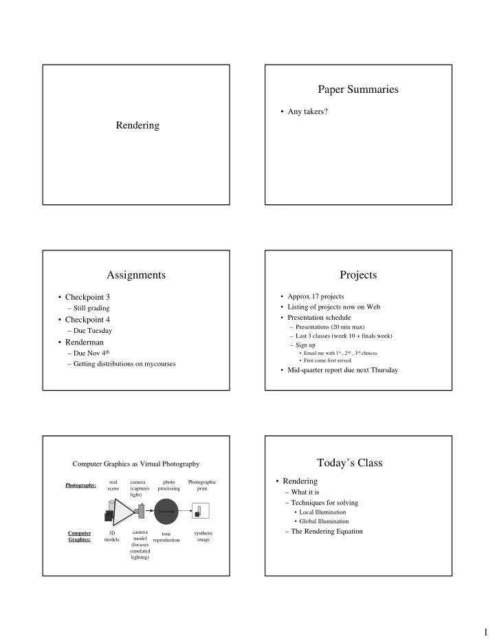
Computer Graphics as Virtual Photography

camera (captures light) synthetic image camera model (focuses simulated lighting)

processing

photo processing tone reproduction real scene 3D models Photography: Computer Graphics: Photographic print

Today’s Class

• Rendering

– What it is – Techniques for solving

• Local Illumination
• Global Illumination

– The Rendering Equation

2

Rendering

• See Render

Render

• (v.) To make visible the final result.
• Aka Shading.

Shading

• Computing the light that leaves a point
• Shading point - point under investigation
• Illumination model - function or algorithm

used to describe the reflective characteristics of a given surface.

• Shading model – algorithm for using an

illumination model to determine the color of a point on a surface.

Shading Models

• Illumination vs. Shading Models

– Each of the illumination models given last class could be applied by either a local or global shading algorithm – The illumination models are not global vs. local, the illumination algorithms are.

• Shading models are examples of local illumination

algorithms.

Shading

• Goal: Determine the color at each pixel

Rasterization

• Visible Surface Determination

– Determine what is rendered where – Done in 2D camera space – Image precision vs object precision

• Image Precision – determine for each pixel, which
• bject is visible at the pixel
• Object Precision – determine for each object, which

part of the object is potentially visible.

3 Image Precision AFTER Projection

For each pixel in image { O = object that is closest draw pixel with appropriate color from O }

Object Precision – BEFORE projection

For each object in scene { determine which parts of object not obscured shade these parts }

Z-buffer

• Visible surface algorithm to determine what
• bject appears on a given pixel

– Image Precision Algorithm – Two frame buffers

• One contains colors
• One contains depth values (Z-buffer)

– Basic idea

• Only calculate shading on object if depth is closer to

value at z-buffer

Z-buffer

• Basic algorithm

Initialize frame buffer (to background) Initialize Z-buffer (to 0) For each polygon P { For each pixel p in polygon’s projection { z = P’s z at pixel p if (z > Zbuffer at that pixel) { zBuffer at pixel = z Frame buffer at pixel = calcColor() } }

Z-buffer

• Applet

http://www.cs.technion.ac.il/%7Ecs234325/Homepage/A pplets/applets/zbuffer/GermanApplet.html

List Priority Algorithms

• Object precision and image-precision

– Sort polygons by z – Rasterize each polygon in order – Problems:

• Polygons must not overlap in z
• If they do, they must be split

4

Shading models

Interpolation

Scan line p1 p2 p3

Shading Models

• Direct Shading Models

– Only consider direct lighting from light sources – Flat (constant) shading – Gouraud Shading – Phong Shading

Shading Models

• Geometry

N H S V R

reflection viewer normal Half-way source

Phong Illumination Model

specular diffuse ambient

V) R ( N) S ( ) (

∑ ∑

• +
• +

=

i k i i s i i i d a a

e

L k L k L k V L

Note: Ln are radiance terms, include both light and material info

Shading Models

• Flat Shading

– Illumination model applied once per polygon. – Constant color for entire polygon – Assumes normal vector is constant across the entire polygon

Shading Models

• Flat shading

Hwang

5

Shading Models

• Gouraud Shading

– Illumination is interpolated across each polygon – Normals required at each polygon vertex, calculated as an average of the normals of each face that shares that vertex – Illumination is calculated for each polygon vertex – Interior points interpolated from endpoint illumination intensities

Shading Models

• Gouraud Shading – finding the normal

Shading Model

• Gouraud Shading

Hwang

Gouraud Rendering Pipeline with Z Buffer

Database traversal Model transform Culling Lighting Viewing transform Clipping Projection Rasterization Display

Shading Models

• Phong Shading

– Normal vectors are interpolated across each polygon – Averaged normal (per Gouraud required at each polygon vertex) – Illumination is calculated for each polygon interior point by applying illumination model directly using interpolated normal

Shading Models

• Phong Shading

Hwang

6 Phong Rendering Pipeline with Z-Buffer

Database traversal Model transform Trivial Accept / Reject View transform Clipping Projection Rasterization and lighting Display

Shading models

• Phong vs. Gouraud

Shading Models

– Comparison

Flat Gouraud Phong

To summarize

• Rasterization

– Scan conversion / Interpolation in 2D – Z-buffer

• Local Illumination models

– Only considers first reflection of light with object – No shadows (unless you add them)

• Shading vs. Illumination Models

– A shading model can use any illumination model – Phong was a busy guy!

The Rendering Equation

• Kajiya: 1986
• “Unified context for viewing rendering

algorithms as more or less accurate approximations to the solution of a single equation”

• Expresses the quantity of light

transferred from one point x’ to another x, summed over all points.

The Rendering Equation

• General form

[ ]

∫

′ ′ ′ ′ ′ ′ ′ ′ + ′ ′ = ′

S

x d x x I x x x x x x x g x x I ) , ( ) , , ( ) , ( ) , ( ) , ( ρ ε

Ashdown

7

The Rendering Equation

• Transport Intensity

I(x, x’) = Transport energy or intensity of light passing from point x’ to point x (unoccluded two point transport)

[ ]

∫

′ ′ ′ ′ ′ ′ ′ ′ + ′ ′ = ′

S

x d x x I x x x x x x x g x x I ) , ( ) , , ( ) , ( ) , ( ) , ( ρ ε

The Rendering Equation

• Geometry term

[ ]

∫

′ ′ ′ ′ ′ ′ ′ ′ + ′ ′ = ′

S

x d x x I x x x x x x x g x x I ) , ( ) , , ( ) , ( ) , ( ) , ( ρ ε

g(x, x’) = geometry term = 0, if x is not visible from x’ = 1/d2 otherwise

The Rendering Equation

• Emittance

[ ]

∫

′ ′ ′ ′ ′ ′ ′ ′ + ′ ′ = ′

S

x d x x I x x x x x x x g x x I ) , ( ) , , ( ) , ( ) , ( ) , ( ρ ε

ε(x, x′) = light energy emitted from point x′ towards x.

The Rendering Equation

• Scattering

[ ]

∫

′ ′ ′ ′ ′ ′ ′ ′ + ′ ′ = ′

S

x d x x I x x x x x x x g x x I ) , ( ) , , ( ) , ( ) , ( ) , ( ρ ε

ρ(x, x′, x′′) = light energy reflected off point x’ towards point x from light coming from x′′

The Rendering Equation

ρ(x, x’, x’’) = light energy reflected from point x’ towards point x from light coming from x’’, i.e. BRDF

The Rendering Equation

• Incoming = direct + indirect (scattered)

[ ]

∫

′ ′ ′ ′ ′ ′ ′ ′ + ′ ′ = ′

S

x d x x I x x x x x x x g x x I ) , ( ) , , ( ) , ( ) , ( ) , ( ρ ε

indirect direct

) (I gR g I + = ε

8

The Rendering Equation

• In short…

– The transport of light from point x’ to point x is equal to the sum of

• the light emitted from x’ in the direction of x and
• the total light scattered from x’ towards x due to

light from all other surfaces in the scene.

The Rendering Equation The Rendering Equation

• This can be expanded using the Neuman series for

implementation purposes:

… + + + + =

3 2

) ( ) ( ) ( Rg g Rg g Rg g g I ε ε ε ε

• r

∑

∞ =

= ) (

i i

Rg g I ε The Rendering Equation

• Why is this important?

… + + + + =

scattering 3rd 3 scattering 2nd 2 scattering 1st direct

) ( ) ( ) ( Rg g Rg g Rg g g I ε ε ε ε

Rendering methods can be characterized by the number of scatterings considered

The Rendering Equation

• Local vs Global Illumination Models

Local illumination - only considers direct component Global illumination - also considers other scattered component

… + + + + =

scattering 3rd 3 scattering 2nd 2 scattering 1st direct

) ( ) ( ) ( Rg g Rg g Rg g g I ε ε ε ε

The Rendering Equation

• Local Illumination

direct

g I ε =

Only object’s first contact with light is considered. Lighting “simulated” by illumination model used. NOTE: Kajiya does not include ambient light!

9

The Rendering Equation

• Global Illumination

Considers multiple scatterings

• Ray-Tracing
• Radiosity
• Kajiya’s method

… + + + + =

scattering 3rd 3 scattering 2nd 2 scattering 1st direct

) ( ) ( ) ( Rg g Rg g Rg g g I ε ε ε ε

The Rendering Equation

• Drawbacks

– Uses geometric optics, based on light as rays – Phase, diffraction, and transmission through participatory media not considered (i.e., only homogenous refraction considered) – Dependence on wavelength is implied – Not expressed using physical units

• Question: Isn’t I (x, x’) simply radiance at a point?
• Yes! (with the exception of some geometric terms…)
• More when we talk about radiosity

The Rendering Equation

• Summary

– Equation for describing rendering algorithms. – Describes light arriving at a point from another point (and indirectly all other points) – Considers direct light and recursive scattering

Break

• When we return…

– Ways of approximating the solution to the rendering equation… – Don’t touch that dial!

Rendering Methods

• Ray Tracing

– Light rays are traced from the eye, through a viewing plane, into scene – When rays strike an object, further rays are spawned representing reflection and refraction. – These newly spawned rays can strike objects and spawn more rays, etc.

Rendering Methods

• Ray Tracing

Watt/Watt

10

Rendering Methods

• Ray tracing

… + + + + =

scattering 3rd 3 scattering 2nd 2 scattering 1st direct

) ( ) ( ) ( Rg g Rg g Rg g g I ε ε ε ε

Number of scatterings depend

• n recursion depth allowed by

ray tracer

Rendering Method

• Ray Tracing – Examples
• Cheesy Video (in case you missed it the first time)

Rendering Methods

• Radiosity

– The problem with ray tracing

• Great for specular type reflections
• Awful for diffuse reflections.

– Radiosity

• From the guys who brought you Cook-Torrance illumination

model!

• Not quite as elegant as ray tracing
• More physically based

Rendering Methods

• Radiosity

– Based on the theory of heat transfer – Calculate lighting in a steady state – Assumes that all surfaces are perfectly diffuse – Formulates a large systems of linear equations – Solution of these equations give you radiant exitance at each point

Rendering Methods

• Radiosity

– Radiant exitance - radiant flux out dA

dA d M Φ =

Rendering Methods

• Radiosity

– Image is created by using calculated radiant existance values in standard rendering process.

• In essence, radiosity defines a “made to fit” texture

mapping

11

Rendering Methods

• Radiosity

– View dependence vs view independence

• Radiosity provides a view independent solution
• Scene needs to be further rendered from a given

view point.

Rendering Methods

• Radiosity

– Not points -- But patches

• Scene is subdivided into patches
• Radiant exitance will be calculated for each patch

Rendering Methods

• Radiosity

– Patches

[Ashdown94]

Radiosity - Basics

• Basic idea

– Each patch will receive a certain amount of light from the environment – It will reflect fraction back into the environment – Keep track of amount of light reflected back – Continue till all light has been exhasted.

Radiosity - Basics

• Key idea

– Since all objects are perfectly diffuse, we can determine where light is coming from (and going) by simply considering the geometry of the scene. – Calculation of radiant exitance per patch is can be detemined mathematically using a closed form solution.

Rendering Methods

• Radiosity

… + + + + =

scattering 3rd 3 scattering 2nd 2 scattering 1st direct

) ( ) ( ) ( Rg g Rg g Rg g g I ε ε ε ε

Mathematical derivation assumes limit as number of scatterings goes to Infinity

12

Rendering Methods

• Radiosity – Examples
• Video

But does anyone use radiosity in practice

• Glad you asked!

– Bunny (Blue Sky Studios)

Remember BRDFs?

Perfectly diffuse Radiosity Perfectly specular Ray tracing Specular & diffuse Reality

Rendering Methods

• Getting closer to reality

– Ray tracing

• Replace rays with cones/beams
• Distributed ray tracing

– Spawn more rays – Stochastic sampling

• Supplement backward ray tracing with forward ray

tracing (e.g. Photon Mapping)

Rendering Methods

• Getting closer to reality

– Radiosity

• Two path method – combine ray tracing and

radiosity

Rendering Methods

• Kajiya’s solution (Path tracing)

– Much like ray tracing – Determine the path of light that eventually reaches the eye. – Only 1 ray spawned per intersection

• Reflection in specular
• Reflection in diffuse
• Refraction

– Which ray to spawn determined via stochastic sampling.

13

Kajiya’s Method Summary

• Rendering equation

– Mathematical expression of rendering process

• Solutions

– Ray Tracing – Radiosity – Combination of both.

• Questions?

Next time

• Recursive ray tracing…in depth