Points in the plane and loops in space z 1 z 2 z 3 z 4 z 1 z 2 z 3 z - - PowerPoint PPT Presentation

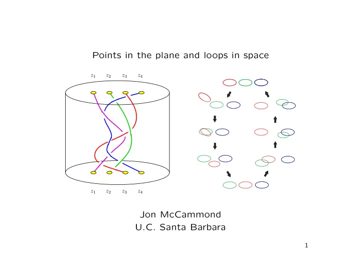
Points in the plane and loops in space

z1 z1 z2 z2 z3 z3 z4 z4

Jon McCammond U.C. Santa Barbara

1

• I. Points in the Plane

z1 z1 z2 z2 z3 z3 z4 z4

2

Geometric group theory Geometric group theorists like it when groups act on metric spaces because, so long as the action is “nice”, the geometry of the space tells you a lot about the group. Nice usually means, by isometries, with a compact quotient, and the action should be free or proper or, at the very least, have understandable stabilizers. A classic example is the fundamental group of a compact metric space acting freely on its universal cover by isometries.

3

The symmetric group Here is a simple example of a group acting on a space. For any field K, the symmetric group Symn acts on the vector space Kn by permuting coordinates. The action is not free since vectors with repeated coordinates are fixed by non-trivial permutations, but it is free on the com- plement of the

n

2

• hyperplanes defined by the equations xi = xj.

This is called the braid arrangement.

4

The real braid arrangement The real braid arrangement is the space of all n-tuples of distinct real numbers (x1, x2, . . . , xn).

x y z

In R3 it consists of 6 connected pieces separated by the planes x = y, x = z and y = z. In Rn it has n! connected pieces separated by the hyperplanes {xi = xj}. The convex hull of the

• rbit of a point is the permutahedron.

5

The complex braid arrangement The complex braid arrangement is the space of all n-tuples of distinct complex numbers (z1, z2, . . . , zn). There is a trick that enables us to visualize this space. The point (z1, z2, z3, z4) = (1 + 3i, 3 − 2i, 0, −2 − i) is encoded in the figure.

Re Im z1 z2 z3 z4

6

The braid group Moving around in the complex braid arrangement corresponds to moving the labeled points in C without letting them collide. Tracing out what happens over time produces braided strings.

z1 z1 z2 z2 z3 z3 z4 z4

The fundamental group of the complex braid arrangement is the pure braid group. The fundamental group of the quotient by the Symn action is the (full) braid group.

7

The Salvetti complex Neither quotient is compact, but they deformation retract onto compact subspaces that can be given cell structures. The Sal- vetti complex for the braid group Braidn is obtained from a permutahedron with an edge orientation induced from a Morse function and an edge coloring invariant under reflections orthog-

• nal to edges. Glue faces with matching labels and orientations.

8

The dual Garside structure Alternatively, here is a very different construction. Minimally factor an n-cycle in Symn into transpositions (closely related to non-crossing partitions). Geometrically realize the resulting

• poset. Finally, glue facets with matching labels and orientations.

1 2 3 4

9

The upshot These two rather different complexes are both Eilenberg-Maclane spaces for the braid groups and either one can be used to calcu- late the homology and cohomology of Braidn. Geometrically, the braid group acts freely and cocompactly by isometries on either universal cover with the permutahedron or the order complex of the noncrossing partition lattice as a fun- damental domain for the action. As a result, there is a close connection between (co)homology calculations for the braid groups, the combinatorics of the per- mutahedron and/or the lattice of non-crossing partitions.

10

• II. Loops in Space

11

Σn and PΣn Our second example is the group of motions of the trivial n-link. Σn is the group of motions of Ln in S3 and PΣn is the index n! subgroup of motions where the n components of Ln return to their original positions. (This is the pure motion group.)

12

Motion groups Let Ln be the trivial n-link in S3, let H(S3) be the space of all self-homeomorphisms of the 3-sphere in the compact-open topology, and let H(S3, Ln) be the subspace of homeomorphisms with φ(Ln) = Ln (preserving circle orientations) for a fixed em- bedding Ln ֒ → S3. A motion of Ln is a path µ : [0, 1] → H(S3) such that µ(0) = the identity and µ(1) ∈ H(S3, Ln). Two motions µ and ν are equivalent if µ−1ν is homotopic to a stationary motion, that is, a motion contained in H(S3, Ln). Introduced by Fox ⇒ Dahm ⇒ Goldsmith · · ·

13

Representing PΣn Thm(Goldsmith, Mich. Math. J. ‘81) There is a faithful representation of PΣn into Aut (F(x1, . . . , xn)) induced by sending the generators of PΣn to automorphisms αij(xk) =

• xk

k = i x−1

j

xixj k = i The image in Aut(Fn) is referred to as the group of pure sym- metric automorphisms since it is the subgroup of automorphisms where each generator is sent to a conjugate of itself. Thinking of PΣn as a subgroup of Aut(Fn) we can form the image of PΣn in Out(Fn), denoted OPΣn.

14

A group by any other name... Four papers, four names, same group.

• “The pure symmetric automorphisms of a free group

form a duality group” (with N. Brady, J. Meier, and A. Miller)

• J. Algebra (2001)
• “The hypertree poset and the ℓ2-Betti numbers of the motion

group of the trivial link” (with J. Meier) Math. Annalen (2004)

• “The integral cohomology of the group of loops” (with C.

Jensen and J. Meier) Geometry and Topology (2006)

• “The Euler characteristic of the Whitehead automorphism

group of a free product” (with C. Jensen and J. Meier) Trans. AMS (2007)

15

McCullough-Miller Complex The computations in these papers are done via an action of OPΣn on a contractible simplicial complex MMn, constructed by McCullough and Miller (MAMS, ‘96). The complex MMn is a space of Fn-actions on simplicial trees, where the actions all take seriously the decomposition of Fn as a free product Fn = Z ∗ · · · ∗ Z

• n copies

. Each action in this space can be described by a marked hypertree.

16

Properties of MMn The McCullough-Miller space, MMn, is the geometric realization

• f a poset of marked hypertrees.

The marking is similar (and related) to the marked graph construction for outer space. Some Useful Facts:

• MMn admits PΣn and OPΣn actions.
• The fundamental domain for either action is the same, it’s

finite and isomorphic to the order complex of HTn (also known as the Whitehead poset).

• The isotropy groups for the OPΣn action are free abelian; the

isotropy groups are free-by-(free abelian) for the action of PΣn.

17

Good News/Bad News The cohomology and/or asymptotic topology of a group G is same as that of the universal cover of a K(G, 1). Good News: We have a contractible, cocompact PΣn-complex. Bad News: The action isn’t free or even proper. Good News: The stabilizers are well understood. Punch Line: The cohomology and/or asymptotic topology of PΣn cannot be directly understood from the cohomology and/or asymptotic topology of MMn because of the bad stabilizers. Instead we plug the combinatorics of HTn and the isotropy groups into arguments involving spectral sequences.

18

Hypertrees A hypertree is a connected hypergraph with no hypercycles. In hypergraphs, the “edges” are subsets of the vertices, not just pairs of vertices. The growth is quite dramatic: The number

• f hypertrees on [n] (due to Smith and Warme,Kalikow), for

n ≥ 3 is = {4, 29, 311, 4447, 79745, 1722681, 43578820, . . .}. The formula is |HTn| =

k nk−1S(n − 1, k) where S(n, k) are Stirling

numbers of the second kind.

1 2 3 4 A= 4 2 1 3 B = 1 2 3 4 C =

19

Exponential generating functions Define the edge weight of a hypertree on [n] as uλ2

2 · · · uλn n

where λi counts the number of edges of size i. Let Tn be the sum of all the weights of hypertrees on [n]. Let Rn be the sum of all the weights of rooted hypertrees on [n]. Let T =

• n

Tn tn n! and let R =

• n

Rn tn n! T3 = u3 + 3u2

2

R3 = 3 · T3 T4 = u4 + 12u2u3 + 16u3

2

R4 = 4 · T4 Thm(Kalikow) R solves the functional equation R = tey where y =

• j≥1

uj+1 Rj j!

20

Drawing conventions Examples of [4]-labelled bipartite trees.

A = 1 2 3 4 C = 1 2 3 4 B = 1 2 3 4 D = 1 2 3 4

Examples of hypertrees on [4].

1 2 3 4 A= 1 2 3 4 C = 4 2 1 3 B = D = 4 1 3 2

21

The hypertree poset The hypertrees on [n] form a very nice poset, that is surprisingly understudied in combinatorics. The elements of HTn are n- vertex hypertrees with the vertices labelled by [n] = {1, . . . , n}. The order relation is given by: τ < τ′ ⇔ each hyperedge of τ′ is contained in a hyperedge of τ. The hypertree with only one edge is 0, also called the nuclear element. If one adds a formal

• 1 such that τ <

1 for all τ ∈ HTn, the resulting poset is HTn.

1 2 3 4 5 6 1 2 3 4 5 6 1 2 3 4 5 6 2 1 3 5 4 6 2 1 3 5 4 6

< < < <

22

First properties of HTn The Hasse diagram of HT4 is

A D D D D

Thm:

• HTn is a finite, graded, bounded lattice.

Pf: Finite, graded, and bounded are easy. Lattice is easy based

• n the similarities between HTn and the partition lattice (and

is the key element in the McCullough-Miller proof that MMn is contractible.)

23

What we do My co-authors and I:

• prove that

HTn is Cohen-Macaulay, and use this to prove that PΣn is a duality group.

• calculate the M¨
• bius function of

HTn and use this to calculate the ℓ2-betti numbers of PΣn.

• calculate Euler characteristics for large classes of groups by

deriving various hypertree identities, and we

• calculate the full integral cohomology of PΣn (including the

ring structure) using the hypertree poset structure to separate the relevant spectral sequences into pieces we can analyze.

24

Cohen-Macaulay A poset is Cohen-Macaulay if its geometric realization is Cohen- Macaulay in the sense that Hi(lk(σ), Z) = 0 for all simplices σ (including the empty simplex) and all i < dim(lk(σ)). (When X is Cohen-Macaulay, this implies that X is homotopy equivalent to a bouquet of spheres.) We show HTn is Cohen-Macaulay by showing that HTn is shellable, which we get by proving HTn admits a recursive atom ordering.

25

The recursive atom ordering Our recursive atom ordering roots the hypertrees at the vertex 1 and then orders by the depth of the vertices (details omitted). Moving around the ordering involves dropping and lifting, and splitting and merging.

6 1 3 4 5 2 5 6 4 2 3 1 lift drop 6 1 3 4 5 1 2 5 6 4 2 split merge 3

26

The M¨

• bius function

Let µ be the M¨

• bius function of

HTn+1 and recall that µ( 0, 1) =

• χ(HT◦

n+1) where the circle indicates that

0 and 1 are removed. Using recursion formulas for M¨

• bius functions, and Kalikow’s

functional equation, we show Thm(M-Meier) µ( 0, 1) = χ(HT◦

n+1) = (−1)nnn−1 .

For example, χ(HT◦

3) = 2,

χ(HT◦

4) = −9,

χ(HT◦

5) = 64.

27

Rooted hypertree and planted hyperforests A rooted hypertree on [12] is shown with its associated planted hyperforest on [11]. One can pass from the hyperforest back to the hypertree using the partition of {1, 3, 5, 6, 8} indicated by the lightly colored boxes.

1 2 3 4 5 6 7 8 9 10 11 12

28

A sample hypertree identity Let the weight of a hyperedge be (e − 1)e−2 where e is its size. Let the weight of vertex i be xval(i)−1

i

where val(i) is its valence. Let the weight of a hypertree be the product of its vertex and edge weights. Thm (Jensen-M-Meier)

• τ∈HTn

Weight(τ) = (x1 + x2 + · · · + xn + n)n−1 This is proved starting with Abel’s identities and a tree result from Stanley. We then prove several partition identities and rooted tree and planted forest identities before reaching this one.

29

• III. Geometric Group Theory

(only if time permitting)

30

Duality groups Def: (Bieri-Eckmann, Invent. Math. ‘73) A group G, with a finite K(G, 1), X, is an n-dimensional duality group if ... H∗

c (

X) = H∗(G, ZG) is torsion-free and concentrated in dim n.

• There is a G-module D such that Hi(G, M) ≃ Hn−i(G, D ⊗ M)

for all i and G-modules M.

• The universal cover

X is (n − 2)-acyclic at infinity. (Geoghegan- Mihalik, JPAA ‘85)

31

Acyclic at infinity Let X be a finite K(π, 1). Then X is m-acyclic at infinity if given any compact C ⊂ X, there is a compact D ⊃ C such that every k-cycle supported in X − D is the boundary of a (k + 1)-chain supported in X − C. (−1 ≤ k ≤ m) Duality groups are groups which are as acyclic at infinity as they can possibly be.

32

Examples of (virtual) duality groups

• Groups like SLn(Z) and SLn(Z[1/p]). (Borel,CMH 1974, Serre,

Topology 1976)

• Mapping class groups of surfaces. (Harer, Invent. Math. 1986)
• Braid groups as well as all Artin groups of finite type. (Squier,
• Math. Scand. 1995, or Bestvina, Geom. & Top. 1999)
• Out(Fn) and Aut(Fn). (Bestvina-Feighn, Invent. Math. 2000)
• PΣn and OPΣn (Brady-M-Meier-Miller, J. Algebra, 2001)

33

Proving duality You can prove that a group is a duality group by showing the cohomology with group ring coefficients is trivial, except in top dimension where it’s torsion-free. The standard equivariant spectral sequence with ZG coefficients for the action of OPΣn on MMn has a complicated first page because the size of the isotropy groups for the action on the poset corresponds with the corank of the elements. It does not correspond well with the dimension of simplices in the geometric realization. On the other hand, the Brown-Meier spectral sequence filters by the poset rank not dimension and collapses immediately when the poset is Cohen-Macaulay. (Brown-Meier, CMH ‘00)

34

ℓ2-cohomology For a group G (admitting a finite K(G, 1)), let ℓ2(G) be the Hilbert space of square-summable functions. The classic cocycle is:

1/2 1/4 1/4 1/4 1/4 1/8 1/8 1/8 1/8 1/8 1/8 1/8 1/8

In general, concrete computations are rare. One of the few is due to Davis and Leary who compute the ℓ2-cohomology of arbitrary right-angled Artin groups (Proc. LMS).

35

ℓ2-betti numbers We compute the ℓ2-betti numbers of OPΣn+1 via its action on MMn+1. In order to do this we have to switch to an alge- braic standpoint, using group cohomology with coefficients in the group von Neumann algebra N(G). We also are really com- puting the equivariant ℓ2-betti numbers of the action of OPΣn+1

• n MMn+1. We can get away with this because
• Lemma. The ℓ2-cohomology of Zn is trivial.

Lemma. Let X be a contractible G-complex. Suppose that each isotropy group Gσ is finite or satisfies b(2)

p

(Gσ) = 0 for p ≥ 0. Then b(2)

p

(X, N(G)) = b(2)

p

(G) for p ≥ 0. (cf. L¨ uck’s L2-Invariants: Theory and Applications ...)

36

Reduction to Euler characteristics In looking at the resulting equivariant spectral sequence we find we are really looking at the homology of HT◦

n+1 = HTn+1 − {the nuclear vertex}

(this is the singular set for the OPΣn+1 action.) Since this poset is Cohen-Macaulay, all we really care about is rank

• Hn−2(HT◦

n+1)

• = |

χ(HT◦

n+1)|

and so computing the ℓ2-betti numbers of the group OPΣn+1 has boiled down to computing the Euler characteristic of the poset HT◦

n+1.

37

Reduction to M¨

• bius functions

To compute χ(HT◦

n+1) we fill up chalk boards with Hasse dia-

grams and compute ... χ(HT◦

3) = 3 = 3

χ(HT◦

4) = 28 − 36 = −8

χ(HT◦

5) = 310 − 855 + 610 = 65, etc.

Luckily, Euler characteristics are well studied in enumerative combinatorics. In particular we can get to the Euler charac- teristic of HT◦

n+1 by studying the M¨

• bius function µ of

HTn+1. Fact: If µ is the M¨

• bius function of
• HTn+1 then µ(

0, 1) =

• χ(HT◦

n+1)

In our case χ(HT◦

3) = 2,

χ(HT◦

4) = −9,

χ(HT◦

5) = 64.

38

The Calculation and Its Corollaries Using recursion formulas for M¨

• bius functions, and Kalikow’s

functional equation, it only takes 3 or 4 pages to show: Thm:

• χ(HT◦

n+1) = (−1)nnn−1 .

Cor 1: The ℓ2-Betti numbers of OPΣn+1 are trivial, except b(2)

n−1 = nn−1. It follows that b(2) n−1(OΣn+1) = nn−1 (n+1)! .

Cor 2: The ℓ2-Betti numbers of PΣn+1 are trivial, except b(2)

n

=

• nn. It follows that b(2)

n

(Σn+1) =

nn (n+1)! .

39