
SLIDE 1
Pool strategy of an electricity producer with endogenous formation - - PowerPoint PPT Presentation
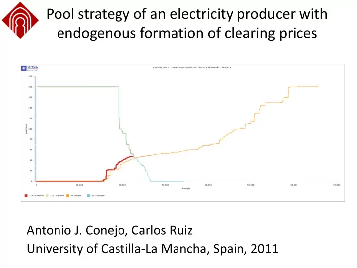
Pool strategy of an electricity producer with endogenous formation of clearing prices Antonio J. Conejo, Carlos Ruiz University of Castilla-La Mancha, Spain, 2011 Contents Background and Aim Approach Model Features Model
29/04/2011 2
29/04/2011 3
29/04/2011 4
29/04/2011 5
4/29/2011 6
Best offering strategy to maximize profit
29/04/2011 7
29/04/2011 8
4/29/2011 9
Social Welfare Maximization (Market Clearing)
Upper-Level Lower-Level
subject to
LMPs Offering curve Dual Variables
11
4/29/2011 12
Upper-Level
LMPs
Offering curve
subject to
13
14
29/04/2011 15
29/04/2011 16
29/04/2011 17
4/29/2011 18
29/04/2011 19
Dual variable
29/04/2011 20
29/04/2011 21
Price
4/29/2011 22
29/04/2011 23
29/04/2011 24
29/04/2011 25
29/04/2011 26
4/29/2011 27
b a
4/29/2011 28
1 , ) 1 ( u M u b uM a b a b a
M Large enough constant (but not too large)
Fortuny-Amat transformation
29/04/2011 29
Based on the strong duality theorem and some of the KKT equalities
29/04/2011 30
29/04/2011 31
4/29/2011 32
S tib
29/04/2011 33
Optimal
curve
4/29/2011 34
To ensure that the final offering curves are increasing in price some additional constraints are needed: These constraints link the individual problems increasing the computational complexity of the model.
4/29/2011 35
4/29/2011 36
4/29/2011 37
29/04/2011 38
29/04/2011 39
29/04/2011 40
29/04/2011 41
4/29/2011 42
The maximum power flow through lines 2-4, 3-6 and 4-6 are 269.62, 229.44 and 39.6933 MW respectively
29/04/2011 43
29/04/2011 44
Capacity of line 3-6 limited to 230 MW:
29/04/2011 45
Capacity of line 3-6 limited to 230 MW:
29/04/2011 46
Capacity of line 4-6 limited to 39 MW:
29/04/2011 47
D tdk
O tjb
29/04/2011 48
29/04/2011 49
Offering curves for strategic generator 1
29/04/2011 50
Offering curves for strategic generator 1
29/04/2011 51
29/04/2011 52
29/04/2011 53
Marginal cost offer Strategic offer
4/29/2011 54
Model 6-bus uncongested 6-bus congested 6-bus stochastic IEEE RTS CPU Time [s] 2.91 5.82 204.77 449.33
29/04/2011 55
– LMPs are endogenously generated: MPEC approach. – Uncertainty is taken into account. – Resulting MILP problem.
29/04/2011 56
29/04/2011 57
Sun Fire X4600 M2 with 4 processors at 2.60 GHz and 32 GB
4/29/2011 58
Model 6-bus uncongested 6-bus congested 6-bus stochastic IEEE RTS CPU Time [s] 2.91 5.82 204.77 449.33
all the producers offer at marginal cost.
4/29/2011 59
29/04/2011 60
29/04/2011 61
29/04/2011 62