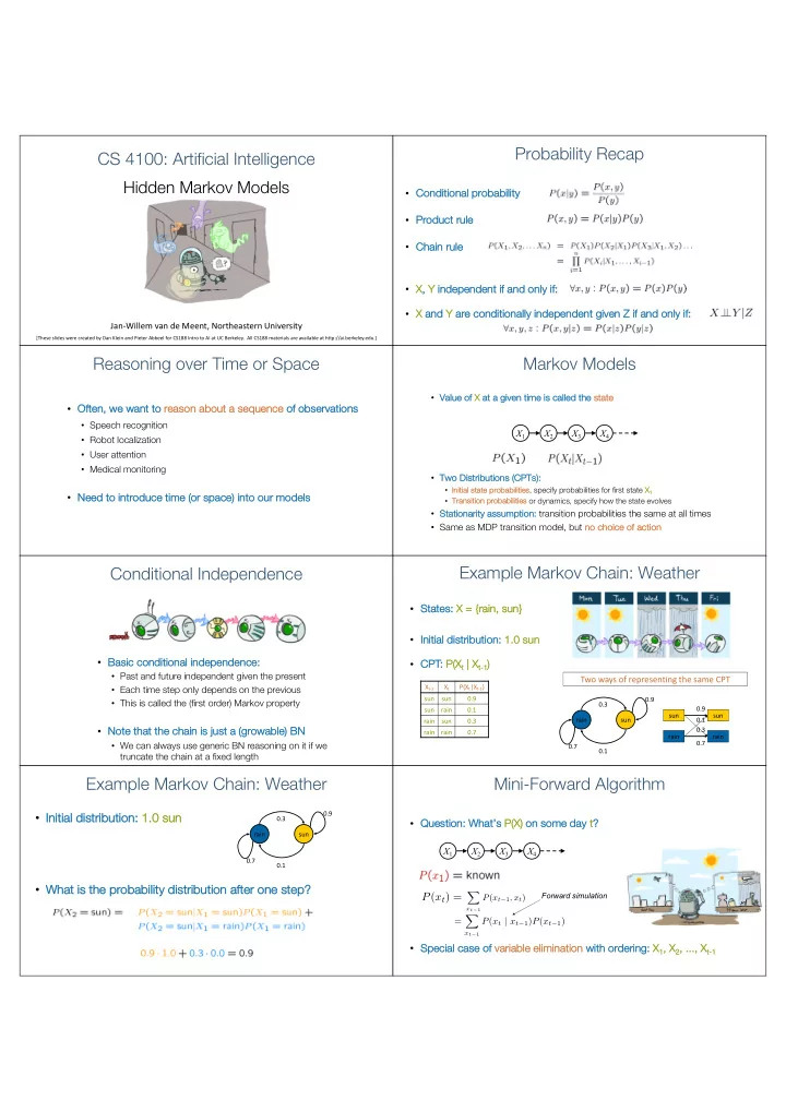
Probability Recap CS 4100: Artificial Intelligence Hidden Markov - - PDF document

probability recap cs 4100 artificial intelligence
SMART_READER_LITE
LIVE PREVIEW

Probability Recap CS 4100: Artificial Intelligence Hidden Markov - - PDF document

Probability Recap CS 4100: Artificial Intelligence Hidden Markov Models Co Conditional probability Pr Product rule Ch Chain rule X, , Y in independent if if and only ly if if: X an and Y ar are co e conditional ally


slide-1
SLIDE 1

CS 4100: Artificial Intelligence Hidden Markov Models

Jan-Willem van de Meent, Northeastern University

[These slides were created by Dan Klein and Pieter Abbeel for CS188 Intro to AI at UC Berkeley. All CS188 materials are available at http://ai.berkeley.edu.]

Probability Recap

  • Co

Conditional probability

  • Pr

Product rule

  • Ch

Chain rule

  • X,

, Y in independent if if and only ly if if:

  • X an

and Y ar are co e conditional ally i indep epen enden ent g given en Z Z i if an and o

  • nly i

if:

Reasoning over Time or Space

  • Oft

Often, we we wa want to re reason

  • n abou

bout a sequ quence of

  • f obs
  • bserv

rvation

  • ns
  • Speech recognition
  • Robot localization
  • User attention
  • Medical monitoring
  • Ne

Need to introduce time me (or sp space) into our mo models

Markov Models

  • Va

Value of X at at a a given en time e is cal called ed the e st state

  • Tw

Two

  • Distr

tributi tion

  • ns (CPTs

Ts):

  • In

Initial s state p probabilities, specify probabilities for first state X1

  • Tra

ransiti tion pr proba babi bilities or dynamics, specify how the state evolves

  • St

Stationarity as assumption: transition probabilities the same at all times

  • Same as MDP transition model, but no

no cho hoice of action X2 X1 X3 X4

Conditional Independence

  • Ba

Basic ic condit itio ional l in independence:

  • Past and future independent given the present
  • Each time step only depends on the previous
  • This is called the (first order) Markov property
  • No

Note that the chain is s just st a (grow growabl ble) ) BN

  • We can always use generic BN reasoning on it if we

truncate the chain at a fixed length

Example Markov Chain: Weather

  • St

States: X X = {ra {rain, sun}

  • In

Initial di distri ribu bution

  • n: 1.

1.0 0 sun

rain sun 0.9 0.7 0.3 0.1

Two ways of representing the same CPT

sun rain sun rain 0.1 0.9 0.7 0.3 Xt-1 Xt P(Xt|Xt-1) sun sun 0.9 sun rain 0.1 rain sun 0.3 rain rain 0.7

  • CP

CPT: P( P(Xt | | Xt-1)

Example Markov Chain: Weather

  • In

Initi tial al di distr tribu buti tion: 1. 1.0 0 sun

  • Wh

What i is t s the p probability d dist stribution a after o

  • ne st

step?

rain sun 0.9 0.7 0.3 0.1

Mini-Forward Algorithm

  • Qu

Question: What’s s P( P(X) on

  • n some
  • me da

day t?

  • Sp

Special case of f va variable elimination wi with ordering: X1, X , X2, ..., X , ..., Xt-1

Forward simulation

X2 X1 X3 X4

P(xt) =

X

xt−1

P(xt−1, xt) = X

xt−1

P(xt | xt−1)P(xt−1)

slide-2
SLIDE 2

Hidden Markov Models Pacman – Sonar (P4) Hidden Markov Models

  • Marko

kov chains not so useful for most agents

  • Need observations to update your beliefs
  • Hidden Marko

kov models (HMMs)

  • Underlying Markov chain over states X
  • You observe outputs (effects) at each time step

X5 X2 E1 X1 X3 X4 E2 E3 E4 E5

Example: Weather HMM

  • An

An HMM is defined by: y:

  • In

Initial al distribution:

  • Tr

Transiti tion

  • ns:
  • Emi

Emissions:

Rt-1 Rt P(Rt|Rt-1) +r +r 0.7 +r

  • r

0.3

  • r

+r 0.3

  • r
  • r

0.7 Umbrellat-1 Rt Ut P(Ut|Rt) +r +u 0.9 +r

  • u

0.1

  • r

+u 0.2

  • r
  • u

0.8 Umbrellat Umbrellat+1 Raint-1 Raint Raint+1

P(Xt | Xt−1) P(Et | Xt)

P(Xt | Xt−1) P(Et | Xt)

Example: Ghostbusters HMM

  • P(

P(X1): uniform

  • P(

P(X X | X’): usually move clockwise, but sometimes move in a random direction or stay in place

  • P(

P(Rij

ij | X

| X): = same sensor model as before; red means close, green means far away.

1/9 1/9 1/9 1/9 1/9 1/9 1/9 1/9 1/9 P(X1) P(X|X’=<1,2>) 1/6 1/6 1/6 1/2

X5 X2 Ri,j X1 X3 X4 Ri,j Ri,j Ri,j

[Demo: Ghostbusters – Circular Dynamics – HMM (L14D2)]

Ghostbusters – Circular Dynamics -- HMM

Conditional Independence

  • HM

HMMs ha have two wo impo portant nt inde ndepe pende ndenc nce pr prope perties:

  • Marko

kov hidden process: future depends on past via the present

  • Current observation in

independent of all else given current state

  • Qu

Quiz: does this mean that evidence variables are guaranteed to be independent?

  • [No, they tend to correlated by the hidden state]

X5 X2 E1 X1 X3 X4 E2 E3 E4 E5

Real HMM Examples

  • Sp

Speech recognition HMMs:

  • Observations are acoustic signals (continuous valued)
  • States are specific positions in specific words (so, tens of thousands)
  • Mach

Machine e tran anslat ation HMMs MMs:

  • Observations are words (tens of thousands)
  • States are translation options
  • Robot tracki

king:

  • Observations are range readings (continuous)
  • States are positions on a map (continuous)
slide-3
SLIDE 3

Filtering / Monitoring

  • Fi

Filtering ng, or monitoring, is the task of tracking the distribution Bt(X) (X) = = Pt(Xt | | e1, …, …, et) (the belief state) over time

  • We start with B1(X

(X) in an initial setting, usually uniform

  • Given Bt(X)

) and new evidence et+

t+1 evidence we compute Bt+ t+1 1 (X)

X)

  • Ba

Basic idea: Use interleaved jo join in, su sum, and no normalize that we have also seen in va variable elimi minati tion:

  • Jo

Join P( P(Xt+

t+1, X

, Xt-1

1 | e

| e1, …, …, et)

  • Su

Sum P( P(Xt+1

1 | e

| e1, …, …, et)

  • Jo

Join P(e (et+

t+1, X

, Xt+1

+1 | e

| e1, …, …, et, et+

t+1)

  • No

Normaliz lize P( P(Xt+

t+1 1 | e

| e1, …, …, et, et+

t+1)

  • The Ka

Kalman f filter r was invented in the 60’s and first implemented as a method of trajectory estimation for the Apollo program

Example: Robot Localization

t=0

  • Se

Sensor mo model: can read in which directions there is a wall, never more than 1 mistake

  • Mo

Motion model el: may not execute action with small prob.

1 Prob

Example from Michael Pfeiffer

Example: Robot Localization

t=1 Li Light hter grey: was possible to get the reading, but less likely b/c required 1 mistake

1 Prob

Example: Robot Localization

t=2

1 Prob

Example: Robot Localization

t=3

1 Prob

Example: Robot Localization

t=4

1 Prob

Example: Robot Localization

t=5

1 Prob

Inference: Base Cases

E1 X1 X2 X1

slide-4
SLIDE 4

Filtering (join + sum): Elapse Time

  • As

Assume me we have ve current belief P( P(X | evi vidence to date)

  • Th

Then, afte fter on

  • ne ti

time ste tep passes:

  • Ba

Basic idea: beliefs get “pushed” through the transitions

  • With the “B” notation, we have to be careful about what time step t

the belief is about, and what evidence it includes

X2 X1 = X

xt

P(Xt+1, xt|e1:t) = X

xt

P(Xt+1|xt, e1:t)P(xt|e1:t) = X

xt

P(Xt+1|xt)P(xt|e1:t)

  • Or compactly:

B0(Xt+1) = X

xt

P(X0|xt)B(xt)

P(Xt+1|e1:t)

Example: Passage of Time

  • As time passes, uncertainty “accumulates”

T = 1 T = 2 T = 5

(Transition model: ghosts usually go clockwise)

Filtering (join + normalize): Observation

  • As

Assume me we have ve current belief P( P(X | previ vious evi vidence):

  • Th

Then, afte fter evidence com

  • mes in:
  • Or

Or, compa pactly: E1 X1

B0(Xt+1) = P(Xt+1|e1:t) P(Xt+1|e1:t+1) = P(Xt+1, et+1|e1:t)/P(et+1|e1:t) ∝Xt+1 P(Xt+1, et+1|e1:t) = P(et+1|Xt+1)P(Xt+1|e1:t) = P(et+1|e1:t, Xt+1)P(Xt+1|e1:t)

B(Xt+1) ∝Xt+1 P(et+1|Xt+1)B0(Xt+1)

  • Ba

Basic idea: beliefs “reweighted” by likelihood of evidence

  • Unlike passage of time, we have

to renormalize

Example: Observation

  • As we get observations, beliefs get reweighted, uncertainty “decreases”

Before observation After observation

B(Xt+1) ∝Xt+1 P(et+1|Xt+1)B0(Xt+1)

First compute pr produ duct (jo (join in) then no normalize

Pacman – Sonar (P4)

[Demo: Pacman – Sonar – No Beliefs(L14D1)]

Pacman – Sonar (with beliefs) Particle Filtering Particle Filtering

0.0 0.1 0.0 0.0 0.0 0.2 0.0 0.2 0.5

  • Fi

Filtering ng: approximate solut ution

  • So

Some metime mes |X |X| is is too big ig to use exact in infere rence

  • |X

|X| may be too big to even store B( B(X)

  • E.g. X is continuous
  • So

Solution: approxima mate inference

  • Track samples of X, not all values
  • Assign weights w

w to all samples (as in likelihood weighting)

  • Weighted samples are called pa

particles

  • In

In me memo mory: list of particles, not states

  • This is how robot localization works

ks in practice

slide-5
SLIDE 5

Representation: Particles

  • Ou

Our repr presentation of P( P(X) is is now a lis list of N pa particles (s (sampl ples)

  • Generally, N <<

<< |X|

  • Storing map from X to counts would defeat the point
  • P(

P(x) approximated by number of particles with value x

  • So, many x may have P(x) =

= 0!

  • More particles, more accuracy
  • For now, all particles have a weight w of 1

Particles: x=(3,3) w=1 x=(2,3) w=1 x=(3,3) w=1 x=(3,2) w=1 x=(3,3) w=1 x=(3,2) w=1 x=(1,2) w=1 x=(3,3) w=1 x=(3,3) w=1 x=(2,3) w=1

Particle Filtering: Elapse Time

  • Mo

Move e each each pa particle is moved d by by sampl pling it its ne next position n from the he trans nsition n model

  • Thi

This s is s like ke pr prior sam sampling ng – probable samples

  • ccur more often, improbable samples less often
  • Here, most samples move clockwise, but some

move in another direction or stay in place

  • Th

This captu tures th the passage ge of

  • f ti

time

  • If enough samples, close to exact values

before and after (consistent)

Particles: x=(3,3) w=1 x=(2,3) w=1 x=(3,3) w=1 x=(3,2) w=1 x=(3,3) w=1 x=(3,2) w=1 x=(1,2) w=1 x=(3,3) w=1 x=(3,3) w=1 x=(2,3) w=1 Particles: x=(3,2) w=1 x=(2,3) w=1 x=(3,2) w=1 x=(3,1) w=1 x=(3,3) w=1 x=(3,2) w=1 x=(1,3) w=1 x=(2,3) w=1 x=(3,2) w=1 x=(2,2) w=1

  • Slightly tricki

kier:

  • Don’t sample observation, fix it
  • Similar to like

kelihood we weig ightin ing, assign weight based on evidence

  • As before, the probabilities don’t sum to one,

since all have been weighted –– in fact, the average weight approximates p( p(e)

Particle Filtering: Observe

Particles: x=(3,2) w=.9 x=(2,3) w=.2 x=(3,2) w=.9 x=(3,1) w=.4 x=(3,3) w=.4 x=(3,2) w=.9 x=(1,3) w=.1 x=(2,3) w=.2 x=(3,2) w=.9 x=(2,2) w=.4 Particles: x=(3,2) w=1 x=(2,3) w=1 x=(3,2) w=1 x=(3,1) w=1 x=(3,3) w=1 x=(3,2) w=1 x=(1,3) w=1 x=(2,3) w=1 x=(3,2) w=1 x=(2,2) w=1

Particle Filtering: Resample

  • Rather than tracki

king weighted samples, we we pe perform re resamplin ling

  • Id

Idea: ea: Preform “natural selection” on particles

  • Sa

Sampl ple new pa particles (with replacement) from

  • ld particles with probability proportional to w
  • Se

Set new weight to 1

  • Hig

igh we weig ight particles will be cloned multiple times

  • Low
  • w weight

ght particles will be eliminated

  • This is equivalent to renormalizing the

distribution

  • Now the update is complete for this time step,

continue with the next one

Particles: x=(3,2) w=.9 x=(2,3) w=.2 x=(3,2) w=.9 x=(3,1) w=.4 x=(3,3) w=.4 x=(3,2) w=.9 x=(1,3) w=.1 x=(2,3) w=.2 x=(3,2) w=.9 x=(2,2) w=.4 (New) Particles: x=(3,2) w=1 x=(2,2) w=1 x=(3,2) w=1 x=(2,3) w=1 x=(3,3) w=1 x=(3,2) w=1 x=(1,3) w=1 x=(2,3) w=1 x=(3,2) w=1 x=(3,2) w=1

Recap: Particle Filtering

  • Pa

Particles: track we weighted samples rather than an explicit distribution

Particles: x=(3,3) w=1 x=(2,3) w=1 x=(3,3) w=1 x=(3,2) w=1 x=(3,3) w=1 x=(3,2) w=1 x=(1,2) w=1 x=(3,3) w=1 x=(3,3) w=1 x=(2,3) w=1

Elapse Weight Resample

Particles: x=(3,2) w=1 x=(2,3) w=1 x=(3,2) w=1 x=(3,1) w=1 x=(3,3) w=1 x=(3,2) w=1 x=(1,3) w=1 x=(2,3) w=1 x=(3,2) w=1 x= (2,2) w=1 Particles: x=(3,2) w=.9 x=(2,3) w=.2 x=(3,2) w=.9 x=(3,1) w=.4 x=(3,3) w=.4 x=(3,2) w=.9 x=(1,3) w=.1 x=(2,3) w=.2 x=(3,2) w=.9 x=(2,2) w=.4 (New) Particles: x=(3,2) w=1 x=(2,2) w=1 x=(3,2) w=1 x=(2,3) w=1 x=(3,3) w=1 x=(3,2) w=1 x=(1,3) w=1 x=(2,3) w=1 x=(3,2) w=1 x=(3,2) w=1

[Demos: ghostbusters particle filtering (L15D3,4,5)]

Ghostbusters – Moderate Number of Particles Ghostbusters – One Particle Ghostbusters – Huge Number of Particles

slide-6
SLIDE 6

Robot Localization

  • In

In robot local calizat ation:

  • We know the map, but not the robot’s position
  • Observations may be vectors of range finder readings
  • State space and readings are typically continuous (works

basically like a very fine grid) and so we cannot store B(X)

  • Particle filtering is a main technique

Particle Filter Localization (Sonar)

[Video: global-sonar-uw-annotated.avi]

Particle Filter Localization (Laser)

[Video: global-floor.gif]

Robot Mapping

  • SL

SLAM AM: Si Simu multaneous Localiza zation An And Mapping

  • We do not know the map or our location
  • State consists of position AND map!
  • Main techniques: Kalman filtering (Gaussian HMMs)

and particle methods

DP-SLAM, Ron Parr [Demo: PARTICLES-SLAM-mapping1-new.avi]

Particle Filter SLAM – Video 1

[Demo: PARTICLES-SLAM-mapping1-new.avi]

Particle Filter SLAM – Video 2

[Demo: PARTICLES-SLAM-fastslam.avi]

Next Lecture: Machine Learning (Naïve Bayes)