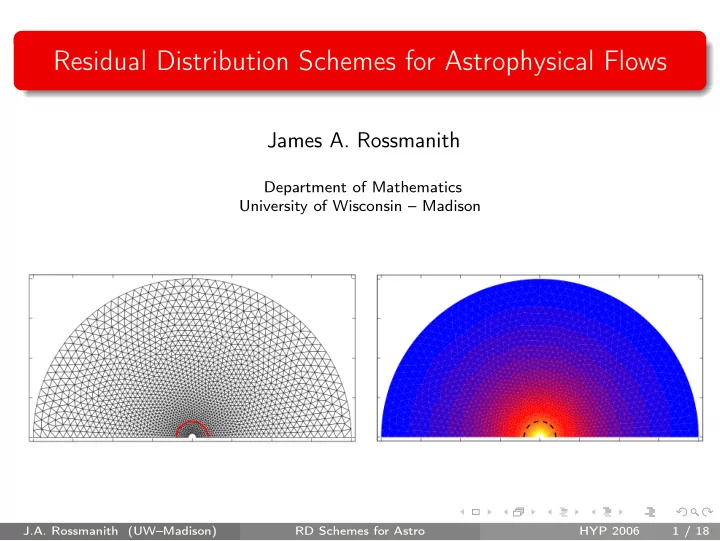
Residual Distribution Schemes for Astrophysical Flows James A. - - PowerPoint PPT Presentation

Residual Distribution Schemes for Astrophysical Flows

James A. Rossmanith

Department of Mathematics University of Wisconsin – Madison

J.A. Rossmanith (UW–Madison) RD Schemes for Astro HYP 2006 1 / 18

Motivation

hubblesite.org lisa.jpl.nasa.gov Astrophysical fluids: black hole accretion, binary black hole interactions Numerical challenges: shocks, geometric singularities, constraints, . . . Numerical methods: FD, spectral, SPH, shock-capturing Goal of this research: develop unstructured, truly multi-D alternative This talk: basic idea & preliminary results on simple equations

J.A. Rossmanith (UW–Madison) RD Schemes for Astro HYP 2006 2 / 18

Why unstructured grids for astrophysics?

Test fluid approximation (fixed metric) Multidimensional balance law “Well-balanced” property needed for a multidimensional balance law Multidimensional (approximate) Riemann solvers Black hole formation and dynamics (time evolving metric) Moving meshes with excised regions inside black holes New black holes may form, old ones may merge = ⇒ change in grid topology

J.A. Rossmanith (UW–Madison) RD Schemes for Astro HYP 2006 3 / 18

Numerical methods on unstructured grids

Discontinuous Galerkin schemes Reed & Hill (1973), Cockburn & Shu (1989) Each element is a control volume Piecewise polynomial in each element 1D Riemann problems at element interfaces RK or space-time time-stepping Residual Distribution schemes Struijs, Deconinck, & Roe (1991), Abgrall (2001) Continuous Petrov-Galerkin method Each dual element is a control volume Multidimensional Riemann problems Good for steady flows, no good version for unsteady

J.A. Rossmanith (UW–Madison) RD Schemes for Astro HYP 2006 4 / 18

Residual distribution schemes

Basic idea: [Roe, 1987], [Deconinck et al., 1993] Hyperbolic balance law: ∂tq + ∇ · F = ψ Solution is stored on nodes of a triangular (tetrahedral) mesh Create residual in each element & distribute to nodes: ΦT ≈ RR

T

h

• ∇ ·

F − ψ i dA = ⇒ ΦT

1 , ΦT 2 , ΦT 3

Update solution by collecting all residuals that influence node i: Qn+1

i

= Qn

i − ∆t |Ci | Σ T :i∈T ΦT i J.A. Rossmanith (UW–Madison) RD Schemes for Astro HYP 2006 5 / 18

Narrow scheme (N-scheme)

3 1 3 2−Target Case 1−Target Case u u 2 2 1 n

2 1

n3 n 1

3 2

n n n

Advection equation: ∂tq + u · ∇q = 0 Narrow scheme: minimal stencil for 1st order, 2D upwind method Residual: Φi = 1

2 [

u · ni]+ (Qi − Q⋆) ≡ βiΦT Conservation: Q⋆ chosen so that P

i Φi = ΦT =

⇒ P

i βi = 1

Monotonicity: N-scheme can be written as Φi = P

j cij(Qi − Qj), where cij ≥ 0

Linear Preserving: improved accuracy in steady-state with βj →

β+

j

P

j β+ j

J.A. Rossmanith (UW–Madison) RD Schemes for Astro HYP 2006 6 / 18

System N-scheme

System N-scheme: Residual: Φi = K +

i (Qi − Q⋆)

Linearization: K( ni) ≡ 1

2

ni · ˆ A( ˆ Q), B( ˆ Q) ˜t = RiΛiLi, K +

i

≡ RiΛ+

i Li

Conservation: Q⋆ chosen so that P

i Φi = ΦT

= ⇒ Q⋆ = "X

i

K +

i

#−1 " ΦT − X

i

K +

i Qi

# The linear preserving condition [Abgrall & Mezine, 2003]: In the system case, Φi = BiφT , where Bi is a matrix Project Φi onto the right e-vectors of K( α) (e.g., α = ˆ u) = ⇒ Φi = P

j βj i

r j Then limit (βj

1, βj 2, βj 3) for each j as in the scalar case =

⇒ (˜ βj

1, ˜

βj

2, ˜

βj

3)

Construct limited residuals: ˜ Φi ≡ P

j ˜

βj

i

r j

J.A. Rossmanith (UW–Madison) RD Schemes for Astro HYP 2006 7 / 18

Compressible Euler equations

∂ ∂t

2 6 6 4 ρ ρu ρv E 3 7 7 5 +

∂ ∂x

2 6 6 4 ρu ρu2 + p ρuv u(E + p) 3 7 7 5 +

∂ ∂y

2 6 6 4 ρv ρuv ρv 2 + p v(E + p) 3 7 7 5 = 0 Equation of state: E =

p γ−1 + 1 2ρ

u2 Waves:

• u · ˆ

n ± c (sound waves),

• u · ˆ

n (entropy wave),

• u · ˆ

n (shear wave) Mach number:

• u/c

J.A. Rossmanith (UW–Madison) RD Schemes for Astro HYP 2006 8 / 18

Example: flow over the NACA 0012 airfoil

Number of elements, nodes: 22,862, 11,618 Number of nodes on outer boundaries, airfoil: 94, 280 Grid is symmetric with respect to y = 0 Grid spacing: hmax ≈ 0.51, hmin ≈ 0.0056

J.A. Rossmanith (UW–Madison) RD Schemes for Astro HYP 2006 9 / 18

Transonic flow over the NACA 0012 airfoil

J.A. Rossmanith (UW–Madison) RD Schemes for Astro HYP 2006 10 / 18

Transonic flow over the NACA 0012 airfoil

J.A. Rossmanith (UW–Madison) RD Schemes for Astro HYP 2006 11 / 18

Astrophysical fluid dynamics

Einstein equations: Rµν − 1 2Rgµν | {z } Spacetime Geometry = 8π Tµν | {z } Matter General description Provides a generalization of Newtonian gravity: ∇2φ = 4πρ Energy-mom., metric, Ricci, scalar curvature: Tµν, gµν, Rµν, R = Rµµ

µ

Four velocity: u = (u0, uj) = (W , v jW ) Lorentz factor: gµνuµuν = −1 = ⇒ W −2 = −g00 − 2g0iv i − gijv iv j Important limits Vacuum limit: Tµν = 0 = ⇒ Rµν = 0 Test fluid limit (mass of fluid ≪ mass of black hole): ∇µT µν = 0 Special relativistic limit (away from massive objects): ds2 = −dt2 + d x2 Newtonian limit ( v ≪ 1): W ≈ 1

J.A. Rossmanith (UW–Madison) RD Schemes for Astro HYP 2006 12 / 18

Test fluid approximation for an ideal gas

∂ ∂x0

@√−g 2 4 D Sj E 3 5 1 A +

∂ ∂xi

@√−g 2 4 ρv iW ρhv iv jW 2 + pg ij ρhv iW 2 + pg i0 3 5 1 A = − 2 4 √−gΓi

µλT µλ

√−gΓ0

µλT µλ

3 5 Covariant formulation [Papadopolous & Font, 2000] q = (D, Sj, E) ≡ (rest-mass, momentum, energy) u = (ρ, v j, p) ≡ (density, fluid 3-velocity, fluid pressure) Specific relativistic enthalpy: h = 1 +

pΓ ρ(Γ−1),

Γ ≡ gas constant Relationship between conserved and primitive variables 2 4 D Sj E 3 5 = 2 4 ρW ρhv jW 2 + pg 0j ρhW 2 + pg 00 3 5 , W = 1 p −g00 − 2g0iv i − gijv iv j Choice of spacetime foliation Spacelike foliations of spacetime (g 00 = 0) = ⇒ Newton iteration for W Null foliations of spacetime (g 00 = 0) = ⇒ no Newton iteration required

J.A. Rossmanith (UW–Madison) RD Schemes for Astro HYP 2006 13 / 18

Schwarzschild black holes

www-gap.dcs.st-and.ac.uk Embedding diagram

Schwarzschild’s solution of the Einstein equations [Schwarzschild, 1916] Assumptions: spherical body with mass M, vacuum outside Black hole: ds2 = − ` 1 − 2M

r

´ dt2 + ` 1 − 2M

r

´−1 dr 2 + r 2dΩ2 2 singularities: event horizon (r = 2M) and black hole (r = 0) Eddington-Finkelstein coordinates The event horizon singularity (r = 2M) can be removed EF time coordinate: dˆ t = dt + “

2M r−2M

” dr EF metric: ds2 = − ` 1 − 2M

r

´ dˆ t2 + 4M

r dˆ

tdr + ` 1 + 2M

r

´ dr 2 + r 2dΩ2

J.A. Rossmanith (UW–Madison) RD Schemes for Astro HYP 2006 14 / 18

Example: radial dust accretion

1 2 5 10 15 0.08 0.16 0.24 0.32 0.4 Density at x0 = 100 [Reg. EF] Exact 201 10

−2

10

−1

10

−10

10

−8

10

−6

10

−4

L1 error as a function of step size p = 2 p = 4 p = 6

Eddington-Finkelstein coordinates: ds2 = − ` 1 − 2M

r

´ dˆ t2 + 4M

r dˆ

t dr + ` 1 + 2M

r

´ dr 2 + r 2dθ2 + r 2 sin2 θ dφ2 Start from constant density state with p ≈ 0, run to steady-state Exact solution known, experimental convergence rate: 2, 4, and 6

J.A. Rossmanith (UW–Madison) RD Schemes for Astro HYP 2006 15 / 18

Example: radial dust accretion

1 2 5 10 15 −0.9 −0.75 −0.6 −0.45 −0.3 v1(x0,x1) at x0 = 100 [Reg. EF] Exact 201 1 2 5 10 15 −6 −4.5 −3 −1.5 v1(x0,x1) at x0 = 100 [Null EF] Exact 201

Null Eddington-Finkelstein coordinates: ds2 = − ` 1 − 2M

r

´ dˆ t2 + 2 dˆ t dr + r 2dθ2 + r 2 sin2 θ dφ2 Start from constant density state with p ≈ 0, run to steady-state Exact solution known

J.A. Rossmanith (UW–Madison) RD Schemes for Astro HYP 2006 16 / 18

Example: radial dust accretion

Cartesian coordinates: x = r cos(θ), y = r sin(θ) Cartesian Eddington-Finkelstein coordinates: det gEF = −r 4 sin2 θ, det gCEF = −r 2 sin2 θ

J.A. Rossmanith (UW–Madison) RD Schemes for Astro HYP 2006 17 / 18

Conclusions and future work

Conclusions

1

RD schemes are an extension of HRSC on unstructured grids

2

Steady flows: conservative & essentially non-oscillatory (shock-capturing)

3

Flexibility for complex geometries (e.g., black holes) Future work

1

High-order non-oscillatory methods

2

RD schemes for time-dependent flows

3

Relativistic magnetohydrodynamics (divergence-free constraint)

4

Simulation of black hole accretion

5

Dynamically evolving spacetimes

J.A. Rossmanith (UW–Madison) RD Schemes for Astro HYP 2006 18 / 18