Review questions BSC3052 FST and PVA 1. Genetic data gives a long - - PDF document

Review questions BSC3052 FST and PVA

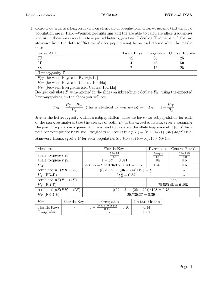
• 1. Genetic data gives a long term view on structure of populations, often we assume that the local

population are in Hardy-Weinberg-equlibrium and the are able to calculate allele frequencies and using those we can calculate expected heterozygosities. Calculate (Recipe below) the two statistics from the data (of ’ficticious’ deer populations) below and discuss what the results mean: Locus ADH Florida Keys Everglades Central Florida FF 92 36 25 SF 4 48 50 SS 2 16 25 Homozygosity F FST [between Keys and Everglades] FST [between Keys and Central Florida] FST [between Everglades and Central Florida] Recipe: calculate F as mentioned in the slides on inbreeding, calculate FST using the expected heterozygosities, in the slides you will see FST = HT − HW HT (this is identical to your notes) → FST = 1 − HW HT HW is the heterozygosity within a subpopulation, since we have two subpopulation for each

• f the pairwise analyses take the average of both, HT is the expected heterozygosity assuming

the pair of population is panmictic: you need to calculate the allele frequency of F (or S) for a pair, for example the Keys and Everglades will result in a p(F) = ((92+4/2)+(36+48/2)/198. Answer: Homozygosity F for each population is : 94/98, (36+16)/100, 50/100 Measure Florida Keys Everglades Central Florida allele frequency pF

92+ 1

24

98 36+ 1

2 48

100 25+ 1

250

100

allele frequency pS 1 − pF = 0.041 04 0.5 HW 2pFpS = 2 × 0.959 × 0.041 = 0.078 0.48 0.5 combined pF(FK − E) ((92 + 2) + (36 + 24))/198 = 7

9

• HT (FK-E)

27

9 2 9 = 0.35

• combined pF(E − CF)
• 0.55

HT (E-CF)

• 20.550.45 = 0.495

combined pF(FK − CF) ((92 + 2) + (25 + 25))/198 = 0.73 HT (FK-CF) 20.730.27 = 0.39 FST Florida Keys Everglades Central Florida Florida Keys

• 1 − (0.078+0.48)/2

0.35

= 0.20 0.34 Everglades

• 0.01

Page: 1

Review questions BSC3052 FST and PVA

• 2. The (ficticious) sightings of Elaphe guttata in Southwood was used to calculate transition

rates from Juveniles to adults (0.255), Staying with the adult class (0.45), having 2 eggs per adult per year.

http://www.uga.edu/srelherp/jd/jdweb/Herps/species/USsnakes/Elagutgut.htm

• Sketch a stage graph, label all parts and fill in the transition rates. Assume that the

transition rates are correct and that the snakes mature within a year.

Juveniles Adults 2 0.255 0.45

• Show the projection matrix,

P =

• 2

0.255 0.45

• calculate the number of juveniles and adults in year 2001 when we use the values of 2000

where we found 30 juveniles and 14 adults. Year Juveniles Adults Total 2000 30 14 44 2001 28 13.95 42

• What is the growth rate between year 2000 and 2001, compare this with the count-based

method above. Growth rate λ = 42

44 [same calculaation as in count based methods once one has summed

up all the stages in a year.]

• Show a graph with time on the x axis and the growth rate λ on the y axis. Calculate λ

for the years 2001 up to 2006 using the start condition (30 juveniles, 14 adults) Page: 2

Review questions BSC3052 FST and PVA Year Juveniles Adults Total 2000 30 14 44 2001 28. 13.95 41.95 2002 27.9 13.4175 41.3175 2003 26.835 13.152375 39.9874 2004 26.30475 12.76149375 39.0662 2005 25.523 12.450 37.97 2006 24.901 12.111 37.012 [I just show the raw table of numbers a figure would include years on the X and numbers

• n the Y, you could plot juveniles and adults or the total. To calculate the growth rate

you divide the numbers in year t by the numbers in year t-1 (for example year 2001 and 2000 λ = 41.95/44) and graph that:

2 3 4 5 6 0.955 0.965 0.97 0.975 0.98 0.985

[Y axis= growth rate, X axis = years: 1 is 2000]

• How would you calculate the stable growth rate? Does your graph give a hint what the

stable growth rate could be? Using the first eigenvalue of the production matrix (this is 0.973749, can be calculated in the program Populus or any other math program: matlab, maple, mathematica, I believe even in Excel). The graph is close and seems to equilibrate around that number.

• Make a prognosis about the population size in year 2007 and 2008.

It will continue to shrink. Page: 3