Simulation of Discrete-Time Markov Chains Discrete-Time Markov - - PowerPoint PPT Presentation

Simulation of Discrete-Time Markov Chains

Peter J. Haas CS590M: Simulation Spring Semester 2020

1 / 13

Simulation of Discrete-Time Markov Chains Discrete-Time Markov Chains (DTMCs) Numerical Solution of DTMCs Simulation of DTMCs Recursive Definition of a DTMC Stationary Distribution of a DTMC General State Space Markov Chains

2 / 13

DTMC Definition

Simplest model for dynamic stochastic system

◮ Xn = system state after nth transition ◮ (Xn : n ≥ 0) satisfies the Markov property

P{Xn+1 = x | Xn = xn, Xn−1 = xn−1, . . . , X0 = x0} = P{Xn+1 = x | Xn = xn}

Time-homogeneous DTMC with state space S defined via

• 1. Transition matrix P = (P(x, y) : x, y ∈ S), with

P(x, y) = P{Xn+1 = y | Xn = x}

• 2. Initial distribution µ = (µ(x) : x ∈ S), with

µ(x) = P {X0 = x}

3 / 13

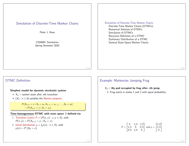
Example: Markovian Jumping Frog

Xn = lily pad occupied by frog after nth jump

◮ Frog starts in states 1 and 2 with equal probability

P =   1/2 1/2 1/3 2/3 3/4 1/4   and µ =   1/2 1/2  

4 / 13

Computing Probabilities and Expectations

Example: θ = P{frog on pad 2 after kth jump}

◮ Write as θ = E[f (Xk)], where f (x) =

• 1

if x = 2

• therwise

◮ Sometimes write indicator function f (x) as I(x = 2) ◮ Q: Why is this correct?

Numerical solution for arbitrary function f

◮ Q: What is probability distribution after first jump? ◮ Let vn(i) = P{frog on pad i after nth jump} vn =

  vn(1) vn(2) vn(3)  

◮ Set v0 = µ and v⊤ m+1 = v⊤ mP for m ≥ 0

I.e., vm+1(j) = 3

i=1 vm(i) P(i, j)

◮ Then E[f (Xk)] = v⊤ k f , where f = [f (1), f (2), f (3)]⊤ ◮ Ex: For θ as above, take f = (0, 1, 0) so that v⊤ k f = v(2)

5 / 13

Simulation of DTMCs

Why simulate? Naive method for generating a discrete random variable

◮ Goal: Generate Y having pmf pi = P{Y = yi} and cdf

ci = P{Y ≤ yi} for 1 ≤ i ≤ m

◮ Example:

i pi ci 1 3/12 3/12 2 8/12 11/12 3 1/12 12/12 3/12 11/12 1 y1 y3 y2

Ex: If U = 0.27, then return Y = y2

◮ Q: How can we speed up this algorithm?

6 / 13

Simulation of DTMCs, Continued

Generating a sample path X0, X1, . . .

• 1. Generate X0 from µ and set m = 0
• 2. Generate Y according to P(Xm, · ) and set Xm+1 = Y
• 3. Set m ← m + 1 and go to 2.

Estimating θ = E[f (Xk)]

• 1. Generate X0, X1, . . . , Xk and set Z = f (Xk)
• 2. Repeat n times to generate Z1, Z2, . . . , Zn (i.i.d.)
• 3. Compute point estimate θn = (1/n) n

i=1 Zi

Can generalize to estimate θ = E[f (W )], where W = f (X0, X1, . . . , Xk)

7 / 13

DTMCs: Recursive Definition

Proposition

◮ Let U1, U2, . . . be a sequence of i.i.d. random variables and X0

a given random variable

◮ (Xn : n ≥ 0) is a time homogeneous DTMC ⇔

Xn+1 = f (Xn, Un+1) for n ≥ 0 and some function f In ⇒ direction, U1, U2, . . . can be taken as uniform Can use to prove that a given process (Xn : n ≥ 0) is a DTMC Q: What if U0, U1, . . . are independent but not identical? Q: Practical advantages of recursive definition?

8 / 13

Example: (s, S) Inventory System

The model

◮ Xn = inventory level at the end of period n ◮ Dn = demand in period n ◮ If (s, S) policy is followed then

Xn+1 =

• Xn − Dn+1

if Xn − Dn+1 ≥ s; S if Xn − Dn+1 < s

Claim: If (Dn : n ≥ 1) is i.i.d. then (Xn : n ≥ 0) is a DTMC with state space {s, s + 1, . . . , S} Q: Critique of model—what might be missing?

9 / 13

Digression: Stationary Distribution of a DTMC

Definition

◮ Informal: π is a stationary distribution of the DTMC if

Xn

D

∼ π implies Xn+1

D

∼ π

◮ Formal:

π(j) = P(Xn+1 = j) =

• i

P(Xn+1 = j | Xn = i) P(Xn = i) =

• i

P(i, j)π(i)

• r π⊤ = π⊤P

◮ So if X0 D

∼ π, then Xn

D

∼ π for n ≥ 1 Under appropriate conditions, limn→∞ P(Xn = i) = π(i)

◮ Also written as Xn ⇒ X, where X D

∼ π How to estimate θ =

i f (i)π(i) = E[f (X)] (where X D

∼ π)?

10 / 13

General State Space Markov Chains: GSSMCs

Problem: With continuous state space, P{Xn+1 = x′ | Xn = x} = 0!

◮ Solution: Use transition kernel

P(x, A) = P{Xn+1 ∈ A | Xn = x}

◮ In practice: Use recursive definition

Example: Continuous (s, S) inventory system Example: Random walk on the real line

◮ Let Y1, Y2, . . . be an i.i.d. sequence of continuous, real-valued

random variables

◮ Set X0 = 0 and Xn+1 = Xn + Yn+1 for n ≥ 0 ◮ Then (Xn : n ≥ 0) is a GSSMC with state space ℜ

11 / 13

GSSMC Example: Waiting times in GI/G/1 Queue

The GI/G/1 Queue

◮ Service center: single server, infinite-capacity waiting room ◮ Jobs arrive one at a time ◮ First-come, first served (FCFS) service discipline ◮ Successive interarrival times are i.i.d. ◮ Successive service times are i.i.d.

Queue Server

12 / 13

GI/G/1 Waiting Times, Continued

Notation

◮ Wn = the waiting time of the nth customer (excl. of service) ◮ An/Dn = arrival/departure time of the nth customer ◮ Vn = processing time of the nth customer

Recursion (Lindley Equation)

◮ Dn = An + Wn + Vn ◮ Thus

Wn+1 = [Dn − An+1]+ = [An + Wn + Vn − An+1]+ = [Wn + Vn − In+1]+

where In+1 = An+1 − An is (n + 1)st interarrival time and [x]+ = max(x, 0)

◮ Thus (Wn : n ≥ 0) is a GSSMC ◮ To simulate: generate the Vn’s and In’s and apply recursion

13 / 13