[PPT] - Spectral analysis of Wikipedia and PhysRev networks Klaus Frahm PowerPoint Presentation

SLIDE 1

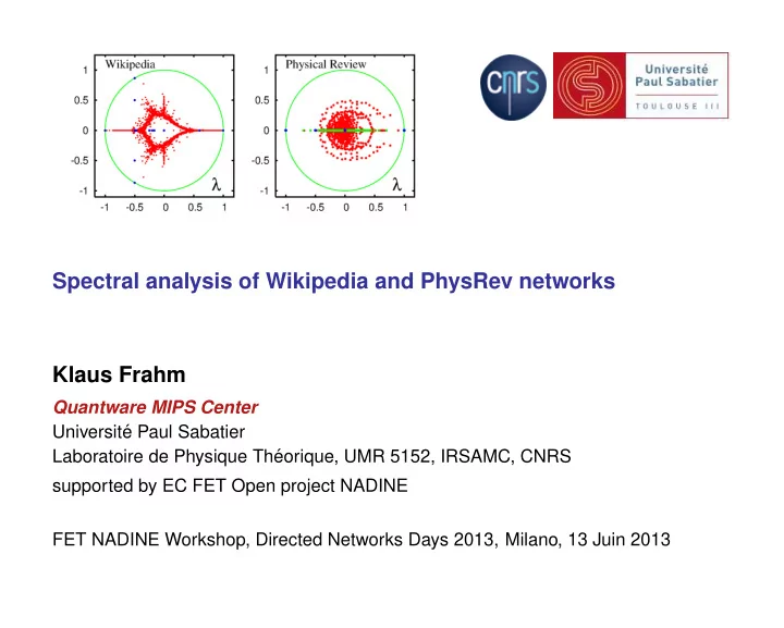
Spectral analysis of Wikipedia and PhysRev networks Klaus Frahm

Quantware MIPS Center Universit´ e Paul Sabatier Laboratoire de Physique Th´ eorique, UMR 5152, IRSAMC, CNRS supported by EC FET Open project NADINE FET NADINE Workshop, Directed Networks Days 2013, Milano, 13 Juin 2013

SLIDE 2

Google matrix for directed networks

Define the adjacency matrix A by Aij = 1 if there is a link from the node j to i in the network (of size N) and Aij = 0 otherwise. Let

Sij = Aij/

i Aij and Sij = 1/N if i Aij = 0 (dangling nodes). S

is of Perron-Frobenius type but for many networks the eigenvalue

λ1 = 1 is highly degenerate [⇒ convergence problem to arrive at the

stationary limit of p(t + 1) = S p(t)]. Therefore define the Google matrix:

G(α) = αS + (1 − α) 1 N eeT

where e = (1, . . . , 1)T and α = 0.85 is a typical damping factor. Here there is a unique eigenvector for λ1 = 1 called the PageRank P and the convergence goes with αt. (CheiRank P ∗ by replacing: A → A∗ = AT).

Klaus Frahm 2 Milano, 13 Juin 2013

SLIDE 3

Arnoldi method

to (partly) diagonalize large sparse non-symmetric d × d matrices:

choose an initial normalized vector ξ0 (random or “otherwise”)
determine the Krylov space of dimension nA (typically:

1 ≪ nA ≪ d ) spanned by the vectors: ξ0, G ξ0, . . . , GnA−1ξ0

determine by Gram-Schmidt orthogonalization an orthonormal

basis {ξ0, . . . , ξnA−1} and the representation of G in this basis:

G ξk =

k+1

j=0

Hjk ξj

diagonalize the Arnoldi matrix H which has Hessenberg form:

H =        ∗ ∗ · · · ∗ ∗ ∗ ∗ · · · ∗ ∗ 0 ∗ · · · ∗ ∗

. . . . . . ... . . . . . .

0 0 · · · ∗ ∗ 0 0 · · · 0 ∗       

which provides the Ritz eigenvalues that are very good aproximations to the “largest” eigenvalues of A.

Klaus Frahm 3 Milano, 13 Juin 2013

SLIDE 4

Invariant subspaces

In realistic WWW or other networks invariant subspaces of nodes create (possibly) large degeneracies of λ1 (or λ2 if α < 1) which is very problematic for the Arnoldi method. Therefore one needs to determine the invariant subspaces defined as subsets of nodes such that for any node in a subspace each

utgoing link stays in the subspace. One can efficiently find all

subspaces of maximal size (or dimension) Nc (with Nc = bN a certain fraction of the network size N, e.g. b = 0.1) and then all subspaces with common members are merged resulting in a decomposition of the network in many separate subspaces with Ns nodes and a “big” core space of the remaining N − Ns nodes. Note that dangling nodes are by construction core space nodes. Possible: core space node → subspace node Impossible: subspace node → core space node

Klaus Frahm 4 Milano, 13 Juin 2013

SLIDE 5

Invariant subspaces

The decomposition in subspaces and a core space implies a block structure of the matrix S:

S =

Sss Ssc

Scc

,

Sss =   S1 0 . . . 0 S2

. . . ...

 

where Sss is block diagonal according to the subspaces. The subspace blocks of Sss are all matrices of PF type with at least one eigenvalue λ1 = 1 explaining the high degeneracies. To determine the spectrum of S apply:

Exact (or Arnoldi) diagonalization on each subspace.
The Arnoldi method to Scc to determine the largest core space

eigenvalues λj (note: |λj| < 1). The largest eigenvalues of Scc are no longer degenerate but other degeneracies are possible (e.g. λj = 0.9 for Wikipedia).

Klaus Frahm 5 Milano, 13 Juin 2013

SLIDE 6

Spectrum of Wikipedia

L. Ermann, KMF and D.L. Shepelyansky, Eur. Phys. J. B 86, 193 (2013)

Wikipedia 2009 : N = 3282257 nodes, Nℓ = 71012307 network links.

spectrum of S, Ns = 515 spectrum of S∗, Ns = 21198

nA = 6000 for both cases

Klaus Frahm 6 Milano, 13 Juin 2013

SLIDE 7

Spectrum of Wikipedia

Some Eigenvectors:

left (right): PageRank (CheiRank) black: PageRank (CheiRank) at α = 0.85 grey: PageRank (CheiRank) at α = 1 − 10−8 red and green: first two core space eigenvectors blue and pink: two eigenvectors with large imaginary part in the eigenvalue

Klaus Frahm 7 Milano, 13 Juin 2013

SLIDE 8

Spectrum of Wikipedia

Detail study of 200 selected eigenvectors with eigenvalues “close” to the unit circle:

Klaus Frahm 8 Milano, 13 Juin 2013

SLIDE 9

Spectrum of Wikipedia

Power law decay of eigenvectors:

|ψi(Ki)| ∼ Kb

i

for

Ki ≥ 104 ϕ = arg(λi)

Klaus Frahm 9 Milano, 13 Juin 2013

SLIDE 10

Spectrum of Wikipedia

Inverse participation ratio of eigenvectors:

ξIPR = (

j |ψi(j)|2)2/ j |ψi(j)|4

ϕ = arg(λi)

Klaus Frahm 10 Milano, 13 Juin 2013

SLIDE 11

Spectrum of Wikipedia

“Themes” of certain eigenvectors:

1
0.5

0.5 1 0.5

0.82
0.8
0.78
0.76
0.74
0.72

0.8 0.82 0.84 0.86 0.88 0.9 0.92 0.94 0.96 0.98 Australia

Switzerland

England Bangladesh New Zeland Poland Kuwait Iceland Austria Brazil China Australia Australia Canada England muscle-artery biology DNA RNA protein skin muscle-artery muscle-artery mathematics math (function, geometry,surface, logic-circuit) rail war

Gaafu Alif Atoll Quantum Leap

Texas-Dallas-Houston

Language music Bible poetry football song poetry aircraft

Klaus Frahm 11 Milano, 13 Juin 2013

SLIDE 12

Spectrum of Wikipedia

Number of links between or inside sets A and B defined by the index

Ki ordered by decreasing absolute value of Wikipedia eigenstates: A = {1, . . . , Ki} B = {Ki + 1, . . . , N}

Klaus Frahm 12 Milano, 13 Juin 2013

SLIDE 13

Physical Review network

(work in progress: KMF , Young-Ho Eom, D. Shepelyansky)

N = 463347 nodes and Nℓ = 4691015 links.

Coarse-grained matrix structure (500 × 500 cells): left: time ordered right: journal and then time ordered “11” Journals of Physical Review: (Phys. Rev. Series I), Phys. Rev., Phys. Rev. Lett., (Rev. Mod. Phys.), Phys. Rev. A, B, C, D, E, (Phys. Rev. STAB and

Phys. Rev. STPER).

Klaus Frahm 13 Milano, 13 Juin 2013

SLIDE 14

Physical Review network

⇒ nearly triangular matrix structure of adjancy matrix: most citations

links t → t′ are for t > t′ (“past citations”) but there is small number (12126 = 2.6 × 10−3Nℓ) of links t → t′ with t ≤ t′ corresponding to future citations. Spectrum by “double-precision” Arnoldi method with nA = 8000: Numerical problem: eigenvalues with |λ| < 0.3 − 0.4 are not reliable! Reason: large Jordan subspaces associated to the eigenvalue λ = 0.

Klaus Frahm 14 Milano, 13 Juin 2013

SLIDE 15

Physical Review network

“very bad” Jordan perturbation theory: Consider a “perturbed” Jordan block of size D:

      0 1 · · · 0 0 0 0 · · · 0 0

. . . . . . ... . . . . . .

0 0 · · · 0 1 ε 0 · · · 0 0      

characteristic polynomial: λD − (−1)Dε

ε = 0 ⇒ λ = 0 ε = 0 ⇒ λj = −ε1/D exp(2πij/D)

for D ≈ 102 and ε = 10−16

⇒

“Jordan-cloud” of artifical eigenvalues due to rounding errors in the region |λ| < 0.3 − 0.4.

Klaus Frahm 15 Milano, 13 Juin 2013

SLIDE 16

Triangular approximation

Remove the small number of links due to “future citations”. Semi-analytical diagonalization is possible:

S = S0 + e d T/N

where en = 1 for all nodes n, dn = 1 for dangling nodes n and

dn = 0 otherwise. S0 is the pure link matrix which is nil-potent: Sl

0 = 0

with l = 352. Let ψ be an eigenvector of S with eigenvalue λ and C = d Tψ.

If C = 0 ⇒ ψ eigenvector of S0 ⇒ λ = 0 since S0 nil-potent.

These eigenvectors belong to large Jordan blocks and are responsible for the numerical problems. Note: Similar situation as in network of integer numbers where l = [log2(N)] and numerical instability for |λ| < 0.01.

Klaus Frahm 16 Milano, 13 Juin 2013

SLIDE 17

Triangular approximation

If C = 0 ⇒ λ = 0 since the equation S0ψ = −C e/N does not

have a solution ⇒ λ1 − S0 invertible.

⇒ ψ = C (λ1 − S0)−1 e/N = C λ

l−1

j=0

S0 λ j e/N . From λl = (d Tψ/C)λl ⇒ Pr(λ) = 0

with the reduced polynomial of degree l = 352 :

Pr(λ) = λl −

l−1

j=0

λl−1−j cj = 0 , cj = d T Sj

0 e/N .

⇒ at most l = 352 eigenvalues λ = 0 which can be numerically

determined as the zeros of Pr(λ). However: still numerical problems:

cl−1 ≈ 3.6 × 10−352
alternate sign problem with a strong loss of significance.
big sensitivity of eigenvalues on cj

Klaus Frahm 17 Milano, 13 Juin 2013

SLIDE 18

Triangular approximation

Solution:

Using the multi precision library GMP with 256 binary digits the zeros of Pr(λ) can be determined with accuracy ∼

10−18.

Furthermore the Arnoldi method can also be implemented with higher precision.

red crosses: zeros of Pr(λ) from 256 binary digits calculation blue squares: eigenvalues from Arnoldi method with 52, 256, 512, 1280 binary digits. In the last case: ⇒ break off at nA = 352 with vanishing coupling element.

Klaus Frahm 18 Milano, 13 Juin 2013

SLIDE 19

Full Physical Review network

High precision Arnoldi method for full Physical Review network (including the “future citations”) for 52, 256, 512, 768 binary digits and

nA = 2000:

Klaus Frahm 19 Milano, 13 Juin 2013

SLIDE 20

Full Physical Review network

Degeneracies

High precision in Arnoldi method is “bad” to count the degeneracy of certain degenerate eigenvalues. In theory the Arnoldi method cannot find several eigenvectors for degenerate eigenvalues, a shortcoming which is (partly) “repaired” by rounding errors.

Q: How are highly degenerate core space eigenvalues possible ?

Klaus Frahm 20 Milano, 13 Juin 2013

SLIDE 21

Full Physical Review network

Semi-analytical argument for the full PR network:

S = S0 + e d T/N

There are two groups of eigenvectors ψ with: Sψ = λψ

1. Those with d Tψ = 0

⇒ ψ is also an eigenvector of S0.

Generically an arbitrary eigenvector of S0 is not an eigenvector of

S unless the eigenvalue is degenerate with degeneracy m > 1.

Using linear combinations of different eigenvectors for the same eigenvalue one can construct m − 1 eigenvectors ψ respecting

d Tψ = 0 which are therefore eigenvectors of S.

Pratically: determine degenerate subspace eigenvalues of S0 (and also of ST

0 ) which are of the form: λ = ±1/√n with

n = 1, 2, 3, . . . due to 2 × 2-blocks:

1/n1

1/n2

⇒

λ = ± 1 √n1 n2 .

Klaus Frahm 21 Milano, 13 Juin 2013

SLIDE 22

Full Physical Review network

2. Those with d Tψ = 0

⇒ R(λ) = 0 with the rational function: R(λ) = 1 − dT 1 λ 1 − S0 e/N = 1 −

j,q

Cjq (λ − ρj)q

Here Cjq and ρj are unknown, except for

ρ1 = 2 Re [(9 + i √ 119)1/3]/(135)1/3 ≈ 0.9024 and ρ2,3 = ±1/ √ 2 ≈ ±0.7071.

Idea: Expand the geometric matrix series ⇒

R(λ) = 1 −

∞

j=0

cjλ−1−j , cj = d T Sj

0 e/N

which converges for |λ| > ρ1 ≈ 0.9024 since cj ∼ ρj

1 for j → ∞.

Problem: How to determine the zeros of R(λ) with |λ| < ρ1 ?

Klaus Frahm 22 Milano, 13 Juin 2013

SLIDE 23

Full Physical Review network

Analytic continuation by rational interpolation: Use the series to evaluate R(z) at nS support points

zj = exp(2πij/nS) with a given precision of p binary digits and

determine the rational function RI(z) which interpolates R(z) at these support points. Two cases:

nS = 2nR + 1 ⇒ RI(z) = PnR(z) QnR(z) nS = 2nR + 2 ⇒ RI(z) = PnR(z) QnR+1(z)

The nR zeros of PnR(z) are approximations of the eigenvalues of

S (of the 2nd group).

For a given precision, e. g. p = 1024 binary digits one can obtain a certain number of reliable eigenvalues, e. g. nR = 300. The method can be pushed up to p = 16384 and nR = 2500 which is better than the high precision Arnoldi method with nA = 2000.

Klaus Frahm 23 Milano, 13 Juin 2013

SLIDE 24

Full Physical Review network

Examples:

Some “artificial zeros” for nR = 340 and p = 1024 (left top and middle panels) where both variants of the method differ. For nR = 300 and p = 1024 most zeros coincide with HP Arnoldi method (right top and middle panels) and both variants of the method coincide. Lower panels: comparison for nR =

2000, p = 12288 (left) or for nR = 2500, p = 16384 with HP Arnoldi

method.

Klaus Frahm 24 Milano, 13 Juin 2013

SLIDE 25

Full Physical Review network

Accurate eigenvalue spectrum for the full Physical Review network by the rational interpolation method (left) and the HP Arnoldi method (right):

Klaus Frahm 25 Milano, 13 Juin 2013

SLIDE 26

Conclusion

Detailed eigenvector study for the Wikipedia network.
Identification of certain themes or communities with the help of

eigenvectors.

Subtle numerical problems for the eigenvalue problem of the

Physical Review network which can be solved by a semi-analytical method and a high precision implementation of the Arnoldi method.

Understanding of the degeneracies of core space eigenvalues

and a decompostion of the core space eigenvalues in two groups. Important role of subspaces of S0 (very different from the subspaces of S !).

Klaus Frahm 26 Milano, 13 Juin 2013

SLIDE 27

Conclusion

New rational interpolation method to determine accurately the

eigenvalues of a network matrix. Well suited for nearly triangular matrices but works in principle also for other case (e. g. Wikipedia but less efficient here).

Drastic effect of the triangular approximation on the eigenvalue
spectrum. Strong reduction of non-vanishing eigenvalues, from

about ∼ 8000 − 10000 to 352 and only very few eigenvalues on the real axis. This implies a very strong effect of the few future citations on the spectrum.

Very useful applications of the GNU high precision library GMP:

http://gmplib.org/ for different numerical methods: determination

f zeros of the reduced polynomial, rational interpolation method,

Arnoldi method.

Klaus Frahm 27 Milano, 13 Juin 2013

SLIDE 28

Conclusion

Appendix:

The subspace of λ = 0 is represented by the vectors

v(j) = Sj−1 e/N for j = 1, . . . , l ⇒ S v(j) = cj−1 v(1) + v(j+1) =

l−1

k=0