The Black-Scholes Model The basic model Two assets: The cash bond - - PowerPoint PPT Presentation

▶

Oct 11, 2023 187 likes •324 views

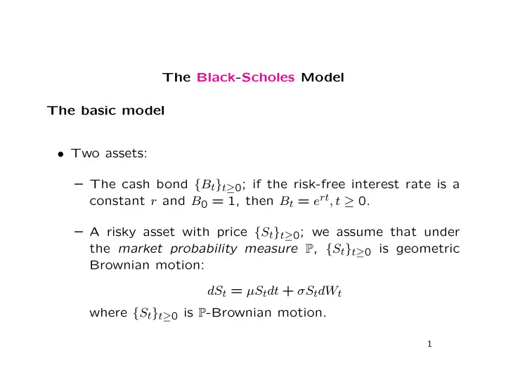
The Black-Scholes Model The basic model Two assets: The cash bond { B t } t 0 ; if the risk-free interest rate is a constant r and B 0 = 1, then B t = e rt , t 0. A risky asset with price { S t } t 0 ; we assume that under

SLIDE 1

The Black-Scholes Model The basic model

Two assets:

– The cash bond {Bt}t≥0; if the risk-free interest rate is a constant r and B0 = 1, then Bt = ert, t ≥ 0. – A risky asset with price {St}t≥0; we assume that under the market probability measure P, {St}t≥0 is geometric Brownian motion: dSt = µStdt + σStdWt where {St}t≥0 is P-Brownian motion.

1

SLIDE 2

Self-financing strategy

We want the no-arbitrage price at time t of a claim CT at

time T that depends on the path up to time T.

If we can replicate the claim with a self-financing portfolio
f cash and stock, the no-arbitrage price must be the value
f that portfolio.
Consider the portfolio (ψ, φ) consisting at time t of ψt bonds

and φt shares; {ψt}0≤t≤T and {φt}0≤t≤T must be predictable.

2

SLIDE 3

To be self-financing, the portfolio value

Vt(ψ, φ) = ψtBt + φtSt satisfies dVt(ψ, φ) = ψtdBt + φtdSt.

In integrated form,

Vt(ψ, φ) − V0(ψ, φ) = ψtBt + φtSt − ψ0B0 − φ0S0 =

t

0 ψudBu +

t

0 φudSu.

That is,

ψtBt + φtSt = ψ0B0 + φ0S0 +

t

0 ψudBu +

t

0 φudSu.

3

SLIDE 4

We assume that

T

0 |ψt|dt +

T

0 |φt|2dt < ∞ :

– ensures that the integrals are well defined; – also excludes strategies, like “doubling”, that require un- bounded borrowing.

If {˜

Vt(ψ, φ)}t≥0 and {˜ St}t≥0 are the corresponding discounted values, then d˜ Vt(ψ, φ) = φtd˜ St,

˜ Vt(ψ, φ) = ˜ V0(ψ, φ) +

t

0 φud˜

Su.

4

SLIDE 5

Approach to pricing the claim

Suppose that we can find a predictable process {φt}0≤t≤T

and a constant φ∗ such that the discounted claim ˜ CT

△

= B−1

T CT

satisfies ˜ CT = φ∗ +

T

0 φud˜

Su.

Note that we do not assume that φ∗ = φ0.

5

SLIDE 6

ψt = φ∗ +

t

0 φud˜

Su − φt ˜ St.

If {˜

Vt(ψ, φ)}0≤t≤T is the value of the portfolio (ψ, φ), then ˜ Vt(ψ, φ) = ψt + φt ˜ St = φ∗ +

t

0 φud˜

Su.

d˜ Vt(ψ, φ) = φtd˜ St, and the portfolio is self-financing.

6

SLIDE 7

Also

˜ VT(ψ, φ) = φ∗ +

T

0 φud˜

Su = ˜ CT, so the portfolio replicates the claim.

So the no-arbitrage price of the claim is

˜ V0(ψ, φ) = φ∗.

Problem: how to find {φt}0≤t≤T and φ∗, or at least φ∗.

7

SLIDE 8

Solution:

find a measure Q such that {˜ St}0≤t≤T is a Q- martingale.

Then so is {˜

Vt(ψ, φ)}0≤t≤T.

φ∗ = ˜ V0(ψ, φ) = EQ ˜ VT(ψ, φ)

= EQ

˜ CT

8

SLIDE 9

The equivalent martingale measure

Recall that

dSt = µStdt + σStdWt so d˜ St = (µ − r)˜ Stdt + σ ˜ StdWt.

Write θ = (µ − r)/σ and Xt = Wt + θt.

9

SLIDE 10

Girsanov’s Theorem states that if Q is defined by

dQ dP

= exp

−θWt − 1

2θ2t

then {Xt}t≥0 is a Q-Brownian motion.
Also

d˜ St = ˜ StσdXt, so {˜ St}t≥0 is a Q-martingale, and ˜ St = ˜ S0 exp

σXt − 1

2σ2t

10

SLIDE 11

The replicating portfolio

We still need to find the predictable processes {ψt}0≤t≤T and

{φt}0≤t≤T defining the replicating portfolio (ψ, φ).

Mt

△

= EQ ˜ CT

Ft
.
Then {Mt}0≤t≤T is a Q-martingale, and by the martingale

representation theorem there exists a predictable process {θt}0≤t≤T such that Mt = M0 +

t

0 θsdXs.

11

SLIDE 12

So if φt = θt/(σ ˜

St), then Mt = M0 +

t

0 φuσ ˜

SudXu = M0 +

t

0 φud˜

Su.

˜ CT = MT = M0 +

T

0 φud˜

Su, as required.

We therefore know that {φt}0≤t≤T exists, but we have not