Today Data Acquisition Systems Many embedded systems measure - - PDF document

1

Today

Data acquisition Digital filters and signal processing

Filter examples and properties FIR filters Filter design Implementation issues DACs PWM

Data Acquisition Systems

Many embedded systems measure quantities from

the environment and turn them into bits

These are data acquisition systems (DAS) This is fundamental

Sometimes data acquisition is the main idea

Digital thermometer Digital camera Volt meter Radar gun

Other times DAS is mixed with other functionality

Digital signal processing Networking, storage Feedback control

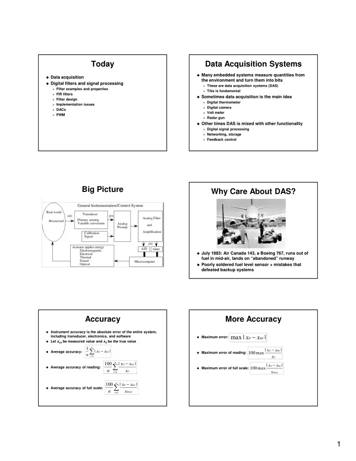
Big Picture Why Care About DAS?

July 1983: Air Canada 143, a Boeing 767, runs out of

fuel in mid-air, lands on “abandoned” runway

Poorly soldered fuel level sensor + mistakes that

defeated backup systems

Accuracy

Instrument accuracy is the absolute error of the entire system,

including transducer, electronics, and software

Let xmi be measured value and xti be the true value Average accuracy: Average accuracy of reading: Average accuracy of full scale:

| | 1

1

• =

−

n i mi ti

x x n

• =

−

n i ti mi ti

x x x n

1

| | 100

• =

−

n i tmax mi ti

x x x n

1

| | 100

More Accuracy

Maximum error: Maximum error of reading: Maximum error of full scale:

| | max

mi ti

x x −

tmax mi ti

x x x | | max 100 −

ti mi ti

x x x | | max 100 −

2

Resolution

Instrument resolution is the smallest input signal

difference that can be detected by the entire system

May be limited by noise in either transducer or electronics

Spatial resolution of the transducer is the smallest

distance between two independent measurements

Determined by size and mechanical properties of the

transducer

Precision

Precision is number of distinguishable alternatives,

nx, from which result is selected

Can be expressed in bits or decimal digits

1000 alternatives: 10 bits, 3 decimal digits 2000 alternatives: 11 bits, 3.5 decimal digits 4000 alternatives: 12 bits, 3.75 decimal digits 10000 alternatives: >13 bits, 4 decimal digits

Range is resolution times precision: rx = x nx

Reproducibility

Reproducibility specifies whether the instrument has

equal outputs given identical inputs over some time period

Specified as full range or standard deviation of

• utput results given a fixed input

Reproducibility errors often come from transducer

drift

ADC: How many bits?

Linear transducer case:

ADC resolution must be problem resolution

Nonlinear transducer case:

Let x be the real-world signal with range rx Let y be the transducer output with range ry Let the required precision of x be nx Resolutions of x and y are x and y Transducer response described by y=f(x) Required ADC precision ny (number of alternatives) is:

• x = rx/nx
• y = min { f(x + x) – f(x) } for all x in rx

Bits is ceiling(log2 ny)

ADC: How many bits?

x ADC must be able to measure a change in voltage of

the smallest y

ADC: How many bits?

x smallest y ADC must be able to measure a change in voltage of

the smallest y

3

DSP Big Picture Signal Reconstruction

Analog filter gets rid of unwanted high-frequency

components in the output

Data Acquisition

Signal: Time-varying measurable quantity whose

variation normally conveys information

Quantity often a voltage obtained from some transducer E.g. a microphone

Analog signals have infinitely variable values at all

times

Digital signals are discrete in time and in value

Often obtained by sampling analog signals Sampling produces sequence of numbers

• E.g. { ... , x[-2], x[-1], x[0], x[1], x[2], ... }

These are time domain signals

Sampling

Transducers

Transducer turns a physical quantity into a voltage ADC turns voltage into an n-bit integer Sampling is typically performed periodically Sampling permits us to reconstruct signals from the world

• E.g. sounds, seismic vibrations

Key issue: aliasing

Nyquist rate: 0.5 * sampling rate Frequencies higher than the Nyquist rate get mapped to

frequencies below the Nyquist rate

Aliasing cannot be undone by subsequent digital

processing

Sampling Theorem

Discovered by Claude Shannon in 1949:

A signal can be reconstructed from its samples without loss of information, if the original signal has no frequencies above 1/2 the sampling frequency

This is a pretty amazing result

But note that it applies only to discrete time, not

discrete values

Aliasing Details

Let N be the sampling rate and F be a frequency

found in the signal

Frequencies between 0 and 0.5*N are sampled properly Frequencies >0.5*N are aliased

• Frequencies between 0.5*N and N are mapped to (0.5*N)-

F and have phase shifted 180

• Frequencies between N and 1.5*N are mapped to f-N with

no phase shift

• Pattern repeats indefinitely

Aliasing may or may not occur when N == F*2*X

where X is a positive integer

4

No Aliasing 1 kHz Signal, No Aliasing Aliasing Avoiding Aliasing

1.

Increase sampling rate

• Not a general-purpose solution
• White noise is not band-limited
• Faster sampling requires:

– Faster ADC – Faster CPU – More power – More RAM for buffering

2.

Filter out undesirable frequencies before sampling using analog filter(s)

• This is what is done in practice
• Analog filters are imperfect and require tradeoffs

Signal Processing Pragmatics Aliasing in Space

Spatial sampling incurs aliasing problems also Example: CCD in digital camera samples an image in

a grid pattern

Real world is not band-limited Can mitigate aliasing by increasing sampling rate

Samples Pixel

5

Point vs. Supersampling

Point sampling 4x4 Supersampling

Digital Signal Processing

Basic idea

Digital signals can be manipulated losslessly SW control gives great flexibility

DSP examples

Amplification or attenuation Filtering – leaving out some unwanted part of the signal Rectification – making waveform purely positive Modulation – multiplying signal by another signal

• E.g. a high-frequency sine wave

Assumptions

1.

Signal sampled at fixed and known rate fs

• I.e., ADC driven by timer interrupts

2.

Aliasing has not occurred

• I.e., signal has no significant frequency components

greater than 0.5*fs

• These have to be removed before ADC using an analog

filter

• Non-significant signals have amplitude smaller than the

ADC resolution

Filter Terms for CS People

Low pass – lets low frequency signals through,

suppresses high frequency

High pass – lets high frequency signals through,

suppresses low frequency

Passband – range of frequencies passed by a filter Stopband – range of frequencies blocked Transition band – in between these

Simple Digital Filters

y(n) = 0.5 * (x(n) + x(n-1))

Why not use x(n+1)?

y(n) = (1.0/6) * (x(n) + x(n-1) + x(n-2) + … + x(n-5) ) y(n) = 0.5 * (x(n) + x(n-3)) y(n) = 0.5 * (y(n-1) + x(n))

What makes this one different?

y(n) = median [ x(n) + x(n-1) + x(n-2) ]

Gain vs. Frequency

Gain

0.0 0.5 1.0 1.5 0.0 0.1 0.2 0.3 0.4 0.5

frequency f/fs

y(n) =(y(n-1)+x(n))/2 y(n) =(x(n)+x(n-3))/2 y(n) =(x(n)+x(n-1))/2 y(n) =(x(n)+x(n-1)+x(n-2)+ x(n-3)+x(n-4)+x(n-5))/6

6

Useful Signals

Step:

…, 0, 0, 0, 1, 1, 1, …

Impulse:

…, 0, 0, 0, 1, 0, 0, …

1

• 3 -2 -1 0

1 2 3 Step s(n) 1 Impulse i(n)

• 1
• 2
• 3

1 2 3

Step Response

1 2 3 4 5 0.2 0.4 0.6 0.8 1 sample number, n step input FIR IIR median Response

Impulse Response

1 2 3 4 5 0.2 0.4 0.6 0.8 1 sample number, n impulse input FIR IIR median Response

FIR Filters

Finite impulse response

Filter “remembers” the arrival of an impulse for a finite time

Designing the coefficients can be hard Moving average filter is a simple example of FIR

Moving Average Example

FIR in C

SAMPLE fir_basic (SAMPLE input, int ntaps, const SAMPLE coeff[], SAMPLE z[]) { z[0] = input; SAMPLE accum = 0; for (int ii = 0; ii < ntaps; ii++) { accum += coeff[ii] * z[ii]; } for (ii = ntaps - 2; ii >= 0; ii--) { z[ii + 1] = z[ii]; } return accum; }

7

Implementation Issues

Usually done with fixed-point How to deal with overflow? A few optimizations

Put coefficients in registers Put sample buffer in registers Block filter

• Put both samples and coefficients in registers
• Unroll loops

Hardware-supported circular buffers

Creating very fast FIR implementations is important

Filter Design

Where do coefficients come from for the moving

average filter?

In general:

1.

Design filter by hand

2.

Use a filter design tool

Few filters designed by hand in practice Filters design requires tradeoffs between

1.

Filter order

2.

Transition width

3.

Peak ripple amplitude

Tradeoffs are inherent

Filter Design in Matlab

Matlab has excellent filter design support

C = firpm (N, F, A) N = length of filter - 1 F = vector of frequency bands normalized to Nyquist A = vector of desired amplitudes

firpm uses minimax – it minimizes the maximum

deviation from the desired amplitude

Filter Design Examples

f = [ 0.0 0.3 0.4 0.6 0.7 1.0]; a = [ 0 0 1 1 0 0]; fil1 = firpm( 10, f, a); fil2 = firpm( 17, f, a); fil3 = firpm( 30, f, a); fil4 = firpm(100, f, a);

fil2 = Columns 1 through 8

• 0.0278 -0.0395 -0.0019 -0.0595 0.0928 0.1250 -0.1667 -0.1985

Columns 9 through 16 0.2154 0.2154 -0.1985 -0.1667 0.1250 0.0928 -0.0595 -0.001 Columns 17 through 18

• 0.0395 -0.0278

Example Filter Response

8

Testing an FIR Filter

Impulse test

Feed the filter an impulse Output should be the coefficients

Step test

Feed the filter a test Output should stabilize to the sum of the coefficients

Sine test

Feed the filter a sine wave Output should have the expected amplitude

Digital to Analog Converters

Opposite of an ADC Available on-chip and as separate modules

Also not too hard to build one yourself

DAC properties:

Precision: Number of distinguishable alternatives

• E.g. 4092 for a 12-bit DAC

Range: Difference between minimum and maximum output

(voltage or current)

Speed: Settling time, maximum output rate

LPC2129 has no built-in DACs

Pulse Width Modulation

PWM answers the question: How can we generate

analog waveforms using a single-bit output?

Can be more efficient than DAC

PWM

Approximating a DAC:

Set PWM period to be much lower than DAC period Adjust duty cycle every DAC period

Important application of PWM is in motor control

No explicit filter necessary – inertia makes the motor its own

low-pass filter

PWM is used in some audio equipment

9

Summary

Filters and other DSP account for a sizable

percentage of embedded system activity

Filters involve unavoidable tradeoffs between

Filter order Transition width Peak ripple amplitude

In practice filter design tools are used We skipped all the theory!

Lots of ECE classes on this