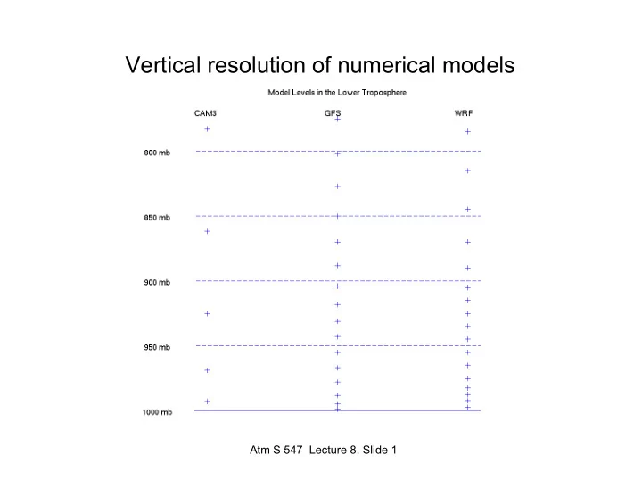
Vertical resolution of numerical models Atm S 547 Lecture 8, Slide - - PowerPoint PPT Presentation

Atm S 547 Lecture 8, Slide 1

Vertical resolution of numerical models

Atm S 547 Lecture 8, Slide 2

M-O and Galperin stability factors

Atm S 547 Lecture 8, Slide 3

Profile vs. forcing-driven turbulence parameterization

Mellor-Yamada turbulence closure schemes are profile-driven: Nonturbulent processes destabilize u,v,θv profiles. è The unstable profiles develop turbulence.

• Such schemes (except 1st order closure) can be numerically delicate:

Small profile changes (e.g. from slightly stable to unstable strat) can greatly change KH,M(z), turbulent fluxes, hence turbulent tendencies. This can lead to numerical instability if the model timestep Δt is large.

• TKE schemes are popular in regional models (Δt ~ 1-5 min).
• Most models use first-order closure for free-trop turbulent layers.

K-profile approach is forcing-driven: KH,M(z) are directly based on surface fluxes or heating rates.

• More numerically stable for long Δt
• Hence K-profile schemes popular in global models (Δt ~ 20-60 min).
• However, K-profile schemes only consider some forcings (e. g.

surface fluxes) and not others (differential advection, internal radiative or latent heating), so can be physically incomplete.

Atm S 547 Lecture 8, Slide 4

K-profile method

• Parameterize turbulent mixing in terms of surface fluxes

(and possibly other forcings) using a specified profile scaled to a diagnosed boundary layer height h.

• Example: Brost and Wyngaard (1978) - for stable BLs

Km(z) = ku*z φm(z L) M-O form     (1− Z)3/2

• h empirically diagnosed using threshold bulk Ri, e. g.

h b(h) − bsfc

( )

u(h) − usfc

( )

2 + v(h) − vsfc

( )

2 +100u* 2 = Ricrit = 0.25

(Z = z/h)

Vogelezang&Holtslag 1996 where ‘sfc’ = 20 m

Atm S 547 Lecture 8, Slide 5

A challenge to downgradient diffusion: Countergradient heat transport

• In dry convective boundary layer, deep eddies transport heat
• This breaks correlation between local gradient and heat flux
• LES shows slight q min at z=0.4h, but w’q’>0 at z<0.8h
• ‘Countergradient’ heat flux for 0.4 < z/h < 0.8…first

recognized in 1960s by Telford, Deardorff, etc.

Cuijpers and Holtslag 1998

CLUBB shines for marine Cu under Sc BLs

Atm S 547 Lecture 8, Slide 6

GCSS ATEX intercomparison case, Bogenschutz et al. 2012 GMD, Fig. 7a

Atm S 547 Lecture 8, Slide 7

Nonlocal schemes This has spawned a class of nonlocal schemes for convective BLs (Holtslag-Boville in CAM3, MRF/ Yonsei in WRF) which parameterize: ( )

a a

a w a K z z γ ∂ ⎛ ⎞ ′ ′ = − − ⎜ ⎟ ∂ ⎝ ⎠

Atm S 547 Lecture 8, Slide 8

Derivation of nonlocal schemes

Heat flux budget:

Holtslag and Moeng (1991)

∂ ∂t ′ w ′ θ = − ′ w ′ w ∂θ ∂z − ∂ ′ w ′ w ′ θ ∂z + g θ0 ′ θ ′ θ − 1 ρ0 ′ θ d ′ p dz

M T

B

P

S

Neglect storage S Empirically:

′ w ′ θ = − τ 2 ′ w ′ w

KH (z)

   ∂θ ∂z + τ w*

2θ*

h

T ≈ B + 2 w*

2θ*

h

P = −aB − ′ w ′ θ τ

For convection, a=0.5, so Take = 0.5h/w* to get zero gradient at 0.4h.

Atm S 547 Lecture 8, Slide 9

Nonlocal parameterization, continued

This has the form ′ w ′ θ = −KH (z) ∂θ ∂z − γ θ ⎛ ⎝ ⎜ ⎞ ⎠ ⎟ γ θ = 2w*

2θ*

′ w ′ w h where Although the derivation suggests is a strong function of z, the parameterization treats it as a constant evaluated at z = 0.4h to obtain the correct heat flux there with d/dz = 0: ′ w ′ w (0.4h) = 0.4w*

2

⇒ γ θ = 5θ* h. The eddy diffusivity can be parameterized from vert. vel. var.:

′ w ′ w (z) = 2.8w*

2Z(1− Z)2,

Z = z h ⇒ KH (z) = 0.7w*z(1− Z)2

With cleverly chosen velocity scales, this can be seamlessly combined with a K-profile for stable BLs to give a generally applicable parameterization (Holtslag and Boville 1993).

Atm S 547 Lecture 8, Slide 10

Comparison of TKE and nonlocal K-profile scheme

UW TKE scheme (Bretherton&Park 2009) vs. Holtslag-Boville.

GABLS1 (Beare et al. 2004)

• Linear initial θ profile
• ug = 10 m/s
• sfc cooled at 0.25K/hr
• 8-9 hr avg profiles
• UW and HB both do well
• Default CAM3 has too

much free-trop diffusion, causing BL overdeepening

Bretherton and Park 2009

Atm S 547 Lecture 8, Slide 11

CBL comparison

• Sfc heating of 300 W m-2
• No moisture or mean wind
• UW TKE scheme with entrainment closure and HB scheme give

similar results at both high and low res.

• Overall, can get comparably good results from TKE and profile-

based schemes on these archetypical cases.

Bretherton and Park 2009