( Y n a bX n ) 2 . n = 1 Thus, Note that E [ X ] = 0 and E [ Y ] - - PowerPoint PPT Presentation

CS70: Lecture 35.

Regression (contd.): Linear and Beyond

• 1. Review: Linear Regression (LR), LLSE
• 2. LR: Examples
• 3. Beyond LR: Quadratic Regression
• 4. Conditional Expectation (CE) and properties
• 5. Non-linear Regression: CE = Minimum Mean-Squared

Error (MMSE)

Review: Linear Regression – Motivation

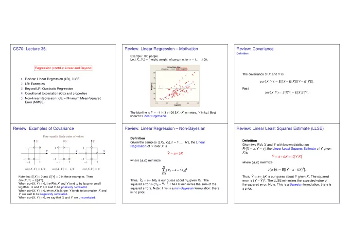
Example: 100 people. Let (Xn,Yn) = (height, weight) of person n, for n = 1,...,100:

E [Y ] Y X

The blue line is Y = −114.3+106.5X. (X in meters, Y in kg.) Best linear fit: Linear Regression.

Review: Covariance

Definition

The covariance of X and Y is cov(X,Y) := E[(X −E[X])(Y −E[Y])]. Fact cov(X,Y) = E[XY]−E[X]E[Y].

Review: Examples of Covariance

Note that E[X] = 0 and E[Y] = 0 in these examples. Then cov(X,Y) = E[XY]. When cov(X,Y) > 0, the RVs X and Y tend to be large or small

• together. X and Y are said to be positively correlated.

When cov(X,Y) < 0, when X is larger, Y tends to be smaller. X and Y are said to be negatively correlated. When cov(X,Y) = 0, we say that X and Y are uncorrelated.

Review: Linear Regression – Non-Bayesian

Definition Given the samples {(Xn,Yn),n = 1,...,N}, the Linear Regression of Y over X is ˆ Y = a+bX where (a,b) minimize

N

∑

n=1

(Yn −a−bXn)2. Thus, ˆ Yn = a+bXn is our guess about Yn given Xn. The squared error is (Yn − ˆ Yn)2. The LR minimizes the sum of the squared errors. Note: This is a non-Bayesian formulation: there is no prior.

Review: Linear Least Squares Estimate (LLSE)

Definition Given two RVs X and Y with known distribution Pr[X = x,Y = y], the Linear Least Squares Estimate of Y given X is ˆ Y = a+bX =: L[Y|X] where (a,b) minimize g(a,b) := E[(Y −a−bX)2]. Thus, ˆ Y = a+bX is our guess about Y given X. The squared error is (Y − ˆ Y)2. The LLSE minimizes the expected value of the squared error. Note: This is a Bayesian formulation: there is a prior.

Review: LR: Non-Bayesian or Uniform?

Observe that 1 N

N

∑

n=1

(Yn −a−bXn)2 = E[(Y −a−bX)2] where one assumes that (X,Y) = (Xn,Yn), w.p. 1 N for n = 1,...,N. That is, the non-Bayesian LR is equivalent to the Bayesian LLSE that assumes that (X,Y) is uniform on the set of

• bserved samples.

Thus, we can study the two cases LR and LLSE in one shot. However, the interpretations are different!

Review: LLSE

Theorem Consider two RVs X,Y with a given distribution Pr[X = x,Y = y]. Then, L[Y|X] = ˆ Y = E[Y]+ cov(X,Y) var(X) (X −E[X]). Non-Bayesian setting: E[X] = 1 N

N

∑

n=1

Xn; E[Y] = 1 N

N

∑

n=1

Yn Var[X] = E[X 2]−(E[X])2 = 1 N

N

∑

n=1

(Xn)2 −( 1 N

N

∑

n=1

(Xn))2 Cov(X,Y) = E[XY]−E[X]E[Y] = 1 N

N

∑

n=1

(XnYn)−( 1 N

N

∑

n=1

Xn)( 1 N

N

∑

n=1

Yn)

LR: Illustration

Note that

◮ the LR line goes through (E[X],E[Y]) ◮ its slope is cov(X,Y) var(X) .

Linear Regression: Examples

Linear Regression: Example 2

We find:

E[X] = 0;E[Y] = 0;E[X 2] = 1/2;E[XY] = 1/2; var[X] = E[X 2]−E[X]2 = 1/2;cov(X,Y) = E[XY]−E[X]E[Y] = 1/2; LR: ˆ Y = E[Y]+ cov(X,Y) var[X] (X −E[X]) = X.

Linear Regression: Example 3

We find:

E[X] = 0;E[Y] = 0;E[X 2] = 1/2;E[XY] = −1/2; var[X] = E[X 2]−E[X]2 = 1/2;cov(X,Y) = E[XY]−E[X]E[Y] = −1/2; LR: ˆ Y = E[Y]+ cov(X,Y) var[X] (X −E[X]) = −X.

Estimation Error

We saw that the LLSE of Y given X is L[Y|X] = ˆ Y = E[Y]+ cov(X,Y) var(X) (X −E[X]). How good is this estimator? That is, what is the mean squared estimation error? We find

E[|Y −L[Y|X]|2] = E[(Y −E[Y]−(cov(X,Y)/var(X))(X −E[X]))2] = E[(Y −E[Y])2]−2(cov(X,Y)/var(X))E[(Y −E[Y])(X −E[X])] +(cov(X,Y)/var(X))2E[(X −E[X])2 = var(Y)− cov(X,Y)2 var(X) . Without observations, the estimate is E[Y] = 0. The error is var(Y). Observing X reduces the error.

Wrap-up of Linear Regression

Linear Regression

• 1. Linear Regression: L[Y|X] = E[Y]+ cov(X,Y)

var(X) (X −E[X])

• 2. Non-Bayesian: minimize ∑n(Yn −a−bXn)2
• 3. Bayesian: minimize E[(Y −a−bX)2]

Beyond Linear Regression: Discussion

Goal: guess the value of Y in the expected squared error

• sense. We know nothing about Y other than its distribution.

Our best guess is? E[Y]. Now assume we make some observation X related to Y. How do we use that observation to improve our guess about Y? Idea: use a function g(X) of the observation to estimate Y. LR: Restriction to linear functions: g(X) = a+bX. With no such constraints, what is the best g(X)? Answer: E[Y|X]. This is called the Conditional Expectation (CE).

Nonlinear Regression: Motivation

There are many situations where a good guess about Y given X is not linear. E.g., (diameter of object, weight), (school years, income), (PSA level, cancer risk). Our goal: explore estimates ˆ Y = g(X) for nonlinear functions g(·).

Quadratic Regression

Let X,Y be two random variables defined on the same probability space. Definition: The quadratic regression of Y over X is the random variable Q[Y|X] = a+bX +cX 2 where a,b,c are chosen to minimize E[(Y −a−bX −cX 2)2]. Derivation: We set to zero the derivatives w.r.t. a,b,c. We get = E[Y −a−bX −cX 2] = E[(Y −a−bX −cX 2)X] = E[(Y −a−bX −cX 2)X 2] We solve these three equations in the three unknowns (a,b,c).

Conditional Expectation

Definition Let X and Y be RVs on Ω. The conditional expectation of Y given X is defined as E[Y|X] = g(X) where g(x) := E[Y|X = x] := ∑

y

yPr[Y = y|X = x].

Deja vu, all over again?

Have we seen this before? Yes. Is anything new? Yes. The idea of defining g(x) = E[Y|X = x] and then E[Y|X] = g(X). Big deal? Quite! Simple but most convenient. Recall that L[Y|X] = a+bX is a function of X. This is similar: E[Y|X] = g(X) for some function g(·). In general, g(X) is not linear, i.e., not a+bX. It could be that g(X) = a+bX +cX 2. Or that g(X) = 2sin(4X)+exp{−3X}. Or something else.

Properties of CE

E[Y|X = x] = ∑

y

yPr[Y = y|X = x] Theorem (a) X,Y independent ⇒ E[Y|X] = E[Y]; (b) E[aY +bZ|X] = aE[Y|X]+bE[Z|X]; (c) E[Yh(X)|X] = h(X)E[Y|X],∀h(·); (d) E[E[Y|X]] = E[Y].

Calculating E[Y|X]

Let X,Y,Z be i.i.d. with mean 0 and variance 1. We want to calculate E[2+5X +7XY +11X 2 +13X 3Z 2|X]. We find E[2+5X +7XY +11X 2 +13X 3Z 2|X] = 2+5X +7XE[Y|X]+11X 2 +13X 3E[Z 2|X] = 2+5X +7XE[Y]+11X 2 +13X 3E[Z 2] = 2+5X +11X 2 +13X 3(var[Z]+E[Z]2) = 2+5X +11X 2 +13X 3.

CE = MMSE

(Conditional Expectation = Minimum Mean Squared Error) Theorem g(X) := E[Y|X] is the function of X that minimizes E[(Y −g(X))2]. That is, E[Y|X] is the ‘best’ guess about Y based on X. Specifically, it is the function g(X) of X that minimizes E[(Y −g(X))2].

Summary

Linear and Non-Linear Regression: Conditional Expectation

◮ Linear Regression: L[Y|X] = E[Y]+ cov(X,Y) var(X) (X −E[X]) ◮ Non-linear Regression: MMSE: E[Y|X] minimizes

E[(Y −g(X))2] over all g(·)

◮ Definition: E[Y|X] := ∑y yPr[Y = y|X = x]