
SLIDE 1
Sampling of ) cos( ) (
0t
t x Ω = at sampling rate
s
Ω
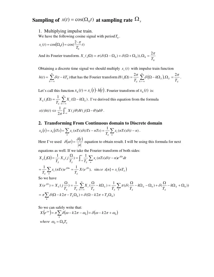
- 1. Multiplying impulse train.
We have the following cosine signal with period T .
( )
) 2 cos( cos ) ( t T t t xc π ⋅ = Ω = And its Fourier transform. 2 )), ( ) ( ( ) ( T j X c π δ δ π = Ω Ω + Ω + Ω − Ω = Ω Obtaining a discrete time signal we should multiply ) (t xc with impulse train function ) ( ) (
S k
kT t t h − = ∑
∞ −∞ =
δ that has the Fourier transform
( )
S S S k S
T k T j H π δ π 2 , 2 ) ( = Ω Ω − Ω = Ω
∑
∞ −∞ =
. Let’s call this function
( ) ( )
t h t x t x
c h
⋅ = ) (
. Fourier transform of
) (t xh
is: ) ( 1 ) (
S k c S h
k X T j X Ω − Ω = Ω
∑
∞ −∞ =
. I’ve derived this equation from the formula θ θ θ π d j H j X t h t x
∫
∞ ∞ −
− Ω ⇔ )) ( ( ) ( 2 1 ) ( ) ( .
- 2. Transforming From Continuous domain to Discrete domain
( ) ( )
∑ ∑
− = − = =
n c S n c h d
n t nTs x T nTs tTs nTs x tTs x t x ) ( ) ( 1 ) ( ) ( δ δ . Here I’ve used ( )
( )
a t at δ δ = equation to obtain result. I will be using this formula for next equations as well. If we take the Fourier transform of both sides:
( ) ( )
S c j S n n j c S t j n c S S h S d
nT x n x ce e X T e nTs x T dt e n t nTs x T T j X T j X = = = − = Ω = Ω
Ω Ω Ω ∞ ∞ −
∑ ∫ ∑
] [ sin ), ( 1 ) ( 1 ) ( ) ( 1 ) ( 1 δ So we have ) 2 ( ) 2 ( )) ( ) ( ( 1 ) ( 1 ) ( ) ( Ω + − Ω + Ω − − Ω = Ω + Ω − Ω + Ω − Ω − Ω = Ω − Ω = Ω =
∑ ∑ ∑
∞ −∞ = Ω S S k S S S S k S S S k c S S h j
T k T k k T k T T k T X T T j X e X π δ π δ π δ δ π So we can safely write that:
( )
( ) ( )
S k j
T where k k e X 2 2 Ω = + − + − − = ∑ ω ω π ω δ ω π ω δ π
ω