Lecture 4 Matthieu Bloch 1 Source coding As shown in Fig. 1, the - - PDF document

Revised December 5, 2019 Information Theoretic Security

Lecture 4

Matthieu Bloch

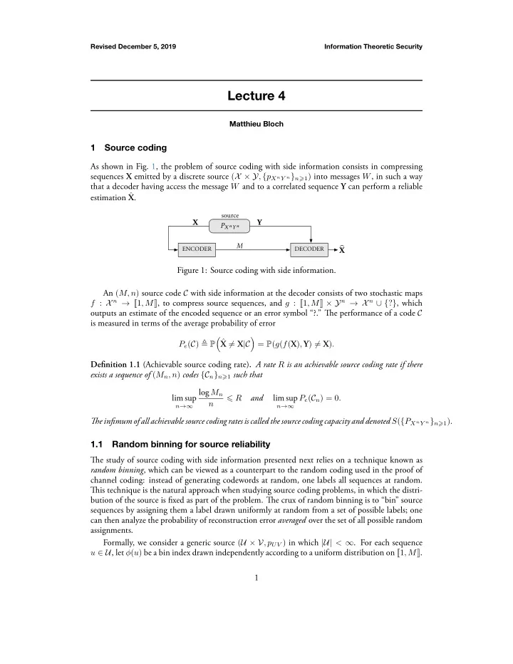
1 Source coding As shown in Fig. 1, the problem of source coding with side information consists in compressing sequences X emitted by a discrete source (X × Y, {pXnY n}n⩾1) into messages W, in such a way that a decoder having access the message W and to a correlated sequence Y can perform a reliable estimation ˆ X.

DECODER ENCODER

! M ! PX nY n

• !

source

Figure 1: Source coding with side information. An (M, n) source code C with side information at the decoder consists of two stochastic maps f : X n → 1, M, to compress source sequences, and g : 1, M × Yn → X n ∪ {?}, which

• utputs an estimate of the encoded sequence or an error symbol “?.” Tie performance of a code C

is measured in terms of the average probability of error Pe(C) ≜ P ( ˆ X = X|C ) = P(g(f(X), Y) = X). Definition 1.1 (Achievable source coding rate). A rate R is an achievable source coding rate if there exists a sequence of (Mn, n) codes {Cn}n⩾1 such that lim sup

n→∞

log Mn n ⩽ R and lim sup

n→∞

Pe(Cn) = 0. Tie infimum of all achievable source coding rates is called the source coding capacity and denoted S({PXnY n}n⩾1).

1.1 Random binning for source reliability Tie study of source coding with side information presented next relies on a technique known as random binning, which can be viewed as a counterpart to the random coding used in the proof of channel coding: instead of generating codewords at random, one labels all sequences at random. Tiis technique is the natural approach when studying source coding problems, in which the distri- bution of the source is fixed as part of the problem. Tie crux of random binning is to “bin” source sequences by assigning them a label drawn uniformly at random from a set of possible labels; one can then analyze the probability of reconstruction error averaged over the set of all possible random assignments. Formally, we consider a generic source (U × V, pUV ) in which |U| < ∞. For each sequence

u ∈ U, let ϕ(u) be a bin index drawn independently according to a uniform distribution on 1, M. 1

Revised December 5, 2019 Information Theoretic Security

For simplicity set K ≜ |U| and U = {ui : i ∈ 1, K}. Tien, if Φ(u) denotes the random variable representing the random mapping of sequence u to an index, we have ∀{ji}K

i=1 ∈ 1, MK

P(Φ(u1) = j1, . . . , Φ(uK) = jK) =

K

∏

i=1

P(Φ(ui) = ji) = ( 1 M )K . For γ > 0, let Bγ = { (u, v) ∈ U × V : log 1 PU|V (u|v) < γ } . Define the encoder as the mapping f : U → 1, M : u → ϕ(u). Define the decoder g : V × 1, M : (v, w) → u∗, where u∗ = u if u is the unique sequence such that (u, v) ∈ Bγ and f(u) = w; otherwise, an error u∗ =? is declared. Tien, the probability of decoding error Pe averaged over the randomly generated bin indices satisfies the following. Lemma 1.2 (Random binning for source reliability). EC(Pe(C)) ⩽ PPUV ((U, V ) / ∈ Bγ) + 2γ M .

• Proof. Let F denote the random variable representing the random indexing function. With succes-

sive applications of the union bound, we obtain E(Pe) = E (∑

u

∑

v

PUV (u, v)1{(u, v) / ∈ Bγ or ∃u′ = u s.t. (u′, v) ∈ Bγ and F(u′) = F(u)} ) ⩽ E (∑

u

∑

v

PUV (u, v)1{(u, v) / ∈ Bγ} ) + E (∑

u

∑

v

PUV (u, v)1{∃u′ = u s.t. (u′, v) ∈ Bγ and F(u′) = F(u)} ) ⩽ PPUV ((u, v) / ∈ Bγ) + E  ∑

u

∑

v

∑

u′̸=u

PUV (u, v)1{(u′, v) ∈ Bγ and F(u′) = F(u)}   = PPUV ((u, v) / ∈ Bγ) + ∑

u

∑

v

∑

u′̸=u

PUV (u, v)1{(u′, v) ∈ Bγ}E(1{F(u′) = F(u)}). For any u′ = u ∈ U, the random binning procedures guarantees that E(1{F(u′) = F(u)}) = P(F(u) = F(u′)) = 1 M . For any (u, v) ∈ Bγ, the definition of Bγ ensures that 1 ⩽ PU|V (u|v)2γ. Consequently, ∀y ∈ Y ∑

u

1{(u, v) ∈ Bγ} ⩽ ∑

u

PU|V (u|v)2γ = 2γ. Notice that the term ∑

u 1{(u, v) ∈ Bγ} is well-defined because |U| < ∞. Tierefore,

E(Pe) ⩽ PPUV ((U, V ) / ∈ Bγ) + ∑

v

PV (v) ∑

u′

1{(u′, v) ∈ Bγ}E(1{F(u′) = F(u)}) ⩽ PPUV ((U, V ) / ∈ Bγ) + 2γ M .

■

2

Revised December 5, 2019 Information Theoretic Security

Using Markov’s inequality, we obtain the following result. Proposition 1.3. Let (U × V, pUV ) be a source. For any M ∈ N∗ and γ > 0, there exists an (M, 1) source code C with deterministic encoder and decoder such that Pe(C) ⩽ PPUV ((U, V ) / ∈ Bγ) + 2γ M . 1.2 Source coding with side information for discrete memoryless sources Definition 1.4 (Discrete Memoryless Source (DMS)). A DMS (X, PX) is a source (X, {PXn}n⩾1) for which PXn is a product distribution, i.e., for any sequence x ∈ X n, we have PXn(x) =

n

∏

i=1

PX(xi). For simplicity, we write P

⊗n

X in place of PXn and S(PX) in place of S({PXn}n⩾1).

Proposition 1.5 (Achievability for source coding with side information). For a DMS (X × Y, PXY ) and any R > H(X|Y ), there exists a sequence {Cn}n⩾1 of (Mn, n) source codes and a constant α > 0 such that lim sup

n→∞

log Mn n ⩽ R and Pe(Cn) ⩽ 2−αn.

• Proof. Tie result follows by applying Lemma 1.2 to the product distribution P

⊗n

XY in place of PUV .

By direct application, we obtain E(Pe(Cn)) ⩽ PP

⊗n

XY

( (X, Y) / ∈ Bn

γ

) + 2γ M . Since P

⊗n

XY is a product distribution,

PP

⊗n

XY

( (X, Y) / ∈ Bn

γ

) = PP

⊗n

XY

( n ∑

i=1

log 1 PX|Y (Xi|Yi) > γ ) . For any δ > 0, upon choosing γ ≜ (1 + δ)H(X|Y ), we obtain PP

⊗n

XY

( n ∑

i=1

log 1 PX|Y (Xi|Yi) > (1 + δ)H(X|Y ) ) ⩽ 2−βn for some β > 0. Hence, choosing the number of bins Mn ≜ ⌊2n(1+2δ)H

(X|Y )⌋, we obtain

E(Pe(Cn)) ⩽ 2−αn for some appropriate choice of α > 0. Finally, we have P(Pe(Cn) > E(Pe(Cn))) < 1 by Markov’s inequality, so that there exists at least one specific sequence of codes {Cn}n⩾1 of (Mn, n) codes for which 1

n log Mn ⩽ (1 + 2δ)H(X|Y ). Hence, (1 + 2δ)H(X|Y ) is an achievable rate, and the result

follows by setting ξ ≜ 2δ. Since ξ > 0 may be chosen arbitrarily small, any rate R > H(X|Y ) is achievable.

■

3

Revised December 5, 2019 Information Theoretic Security

It is also possible to establish a converse result. Proposition 1.6 (Converse for source coding with side information). For a DMS (X × Y, PXY ), any achievable rate must satisfy R ⩾ H(X|Y ) . (1)

• Proof. Consider an (Mn, n) code Cn with probability of error ϵn. Tien,

log Mn ⩾ H(M) ⩾ H(M|Y) ⩾ I(M; X|Y) = H(X|Y) − H(X|MY) ⩾ nH(X|Y ) − 1 − ϵnn log |X| , where the last inequality follows from Fano’s inequality. Consequently, 1 n log Mn ⩾ H(X|Y ) − 1 n − ϵn log |X| . Taking the limit as n → ∞ and ϵn → 0 yields 1

n log Mn ⩾ H(X|Y ).

■

Combining Proposition 1.5 with Proposition 1.6, we obtain the following. Tieorem 1.7 (Source coding with side information for a DMS). For a DMS with two component (X × Y, PXY ), we have S(PXY ) = H(X|Y ) . 2 Channel output approximation Tie problem of channel output approximation (channel approximation for short) is illustrated in Figure 2. Consider a source (X, {PXn}n⩾1) and a channel (X, {WZn|Xn}n⩾1, Z). If the output of the source is used as the input to the channel, the output of the channel is another source (Z, QZn) characterized by ∀z ∈ Zn QZn(z) = ∑

x

PXn(x)WZn|Xn(z|x). Tie objective of channel approximation is to approximate the output statistics QZn using an (Mn, n) channel code in place of the source (X, PXn). If the codewords {xi}i∈1,Mn in the channel code are used uniformly at random, the corresponding output statistics are ∀z ∈ Zn PZn(z) =

Mn

∑

m=1

WZn|Xn(z|xm) 1 Mn . Any distance δ on the space of distributions over Zn is a potential metric to measure how well PZn approximates QZn. We focus here specifically on D(PZnQZn). Definition 2.1 (Achievable channel approximation rate and channel resolvability). A rate R is an achievable approximation rate if there exists a sequence of (Mn, n) channel codes {Cn}n⩾1 such that lim sup

n→∞

1 n log Mn ⩽ R and lim

n→∞ δ(PZn, QZn) = 0.

Tie infimum of all achievable rates is the channel resolvability Cr({WZn|Xn}n⩾1, {PXn}n⩾1). 4

Revised December 5, 2019 Information Theoretic Security

ENCODER

M WZ n |X n WZ n |X n ! ∼ QZ n ! ∼ PX n ! ∼ PZ n

Figure 2: Channel output approximation over a noisy channel. Notice that the notion of channel resolvability is not quite cast as the channel capacity for channel coding because the input distribution PX to the channel that determines the output to approximate is fixed. One could instead ask for the minimum rate of randomness over all possible input processes, but the chosen formulation turns out more useful when discussing information theoretic security. 2.1 Random coding for channel approximation Random coding plays again a central role in indentifying the achievable channel approximation

• rates. Formally, consider a generic source (U, PU) and a generic channel (U, WV |U, V), where the al-

phabets U and V are arbitrary. Let {ui}i∈1,M be codewords obtained as the realizations of M inde- pendent draws according to PU. let QV (v) ≜ ∑

u WV |U(v|u)PU(u), PV (v) ≜ ∑M i=1 WV |U(v|ui) 1 M ,

and for γ > 0 Cγ ≜ { (u, v) ∈ U × V) : log WV |U(v|u) QV (v) ⩽ γ } . Tien, the expected values of D(PV QV ) and V(PV , QV ) over the randomly generated codewords satisfy the following lemmas. Lemma 2.2 (Random coding for D-approximation). For any γ > 0, E(D(PV QV )) ⩽ PPUWV |U ((U, V ) / ∈ Cγ) log ( 1 µV + 1 ) + 2γ M , where µV ≜ minv∈suppQV QV (v).

• Proof. Denote {Ui}i∈1,M the random variables representing the randomly generated codewords.

Denote E∼i the expectation over all Uj with j ∈ 1, M \ {i}. Note that, E(D(PV QV )) =

M

∑

i=1

1 M ∑

v

E ( WV |U(v|Ui) log (∑M

j=1 WV |U(v|Uj)

MQV (v) )) =

M

∑

i=1

1 M ∑

v

∑

ui

WV |U(v|ui)PU(ui)E∼i ( log (∑M

j=1 WV |U(v|Uj)

MQV (v) )) 5

Revised December 5, 2019 Information Theoretic Security

(a)

⩽

M

∑

i=1

1 M ∑

v

∑

ui

WV |U(v|ui)PU(ui) log E∼i (∑M

j=1 WV |U(v|Uj)

MQV (v) ) =

M

∑

i=1

1 M ∑

v

∑

ui

WV |U(v|ui)PU(ui) log (WV |U(v|ui) MQV (v) + M − 1 M )

(b)

⩽ ∑

v

∑

u

WV |U(v|x)PU(u) log (WV |U(v|u) MQV (v) + 1 ) , where (a) follows by Jensen’s inequality and (b) holds because for j = i E∼i ( WV |U(v|Uj) ) = QV (v). If (u, v) ∈ Cγ, notice that log (WV |U(v|u) MQV (v) + 1 ) ⩽ log ( 2γ M + 1 ) ⩽ 2γ M . (2) In contrast, if (u, v) / ∈ Cγ, we have log (WV |U(v|u) MQV (v) + 1 ) ⩽ log ( 1 µV + 1 ) . (3) Hence, E(D(PV QV )) ⩽ PPUWV |U ((U, V ) / ∈ Cγ) log ( 1 µV + 1 ) + 2γ M , (4)

■

Notice that Lemma 2.2 is not useful when µV = 0, which prevents its application for many continuous channels such as Additive White Gaussian Noise (AWGN) channels. 6